|
|
PPCC PLOTName:
... KOLMOGOROV SMIRNOV PLOT ... ANDERSON DARLING PLOT ... CHI-SQUARE PLOT
The PPCC plot is based on the following two ideas:
The PPCC plot is formed by selecting a value of the shape parameter, generating the probability plot (this probability plot is not actually graphed), and then computing the correlation coefficient of the resulting probability plot. The PPCC plot then consists of:
The value of the distributional parameter (on the horizontal axis) which corresponds to the maximum of the PPCC plot curve (on the vertical axis) is, of course, of interest since it indicates the best-fit member of the family. The PPCC PLOT has been extended to support the following additional goodness of fit statistics:
For these alternative measures of goodness of fit, we follow a similar procedure. That is, we fix a value of the shape parameter, generate the corresponding probability plot in the background to obtain estimates for location and scale, and then compute the goodness of fit statistic based on these parameters. For these goodness of fit statistics, we are looking for the minimum value of the statistic rather than the maximum value of the statistic. Some advantages of the PPCC plot as a fitting technique are:
Some disadvantages of the PPCC plot as a fitting technique are:
PPCC plots are available for the following continuous distributional families (with the distributional parameter in parentheses) with one shape parameter:
PPCC plots are available for the following continuous distributional families (with the distributional parameter in parentheses) with two shape parameters:
PPCC plots are available for the following discrete distributional families (with the distributional parameter in parentheses):
The use of the PPCC plot for discrete distributions is still experimental (see the Note below). The percent point function for the discrete distributions is a step function (since X is restricted to integer values). This can result in non-smooth ppcc and probability plots. For discrete distributions, the KS PLOT (which will plot the minimum value of chi-square statistic) is recommended over the PPCC PLOT as long as the sample size is reasonably large.
where <y> is the variable of raw data values under analysis; <family> is one of the distributions listed above; and where the <SUBSET/EXCEPT/FOR qualification> is optional. This syntax is used for the raw data case. The syntax PPCC PLOT can be replaced with ANDERSON DARLING PLOT, KOLMOGOROV SMIRNOV PLOT, or CHI-SQUARE PLOT to generate the Anderson-Darling, Kolmogorov-Smirnov, and chi-square variants of the plot, respectively.
<SUBSET/EXCEPT/FOR/qualification> where <y> is the variable of pre-computed frequencies; <x> is the variable of distinct values for the variable under analysis; <family> is one of the families listed above; and where the This syntax is used for the binned data case where the bins are defined by the mid-points of each bin. The syntax PPCC PLOT can be replaced with CHI-SQUARE PLOT to generate the chi-square variant of the plot. This syntax is not supported for the Anderson-Darling and Kolmogorov-Smirnov variants of the plot.
<SUBSET/EXCEPT/FOR/qualification> where <y> is the variable of pre-computed frequencies; <xlow> is the variable containing the lower limits for the bins; <xhigh> is the variable containing the upper limits for the bins; <family> is one of the families listed above; and where the <SUBSET/EXCEPT/FOR qualification> is optional. This syntax is used for the binned data case where the bins are defined by the lower and upper limits of the bins (i.e., the bins can be of unequal width). The syntax PPCC PLOT can be replaced with CHI-SQUARE PLOT to generate the chi-square variant of the plot. This syntax is not supported for the Anderson-Darling and Kolmogorov-Smirnov variants of the plot.
<SUBSET/EXCEPT/FOR/qualification> where <y> is the variable of raw data values under analysis; <x> is the censoring variabe; <family> is one of the distributions listed above; and where the <SUBSET/EXCEPT/FOR qualification> is optional. This syntax is used for the raw data case where there is censoring. Censoring is not supported for discrete disributions or grouped data. It is also not supported for the Anderson-Darling, Kolmogorov-Smirnov, and chi-square variants of the plot.
<SUBSET/EXCEPT/FOR/qualification> where <y> is the variable of raw data values under analysis; <censor> is the censoring variabe; <x> is the variable of distinct values for the variable under analysis; <family> is one of the distributions listed above; and where the <SUBSET/EXCEPT/FOR qualification> is optional.
This syntax is used for the case where we have frequency (binned)
data with censoring. The bins are defined by their mid-points.
When a particular bin has both censored and uncensored data,
there will be 2 rows with the same value for
A value of 1 indicates a failure time and a value of 0 indicates
a censoring time.
Censoring is not supported for discrete disributions or grouped
data. It is also not supported for the Anderson-Darling,
Kolmogorov-Smirnov, and chi-square variants of the plot.
<SUBSET/EXCEPT/FOR/qualification> where <y> is the variable of raw data values under analysis; <censor> is the censoring variabe; <xlow> is the variable containing the lower limits for the bins; <xhigh> is the variable containing the upper limits for the bins; <family> is one of the distributions listed above; and where the <SUBSET/EXCEPT/FOR qualification> is optional. This syntax is used for the case where we have frequency (binned) data with censoring. The bins are defined by their lower and upper limits. This syntax allows bins with unequal widths. When a particular bin has both censored and uncensored data, there will be 2 rows with the same values for <xlow> and <xhigh>. A value of 1 indicates a failure time and a value of 0 indicates a censoring time for the censoring variable. Censoring is not supported for discrete disributions or grouped data. It is also not supported for the Anderson-Darling, Kolmogorov-Smirnov, and chi-square variants of the plot.
<SUBSET/EXCEPT/FOR/qualification> where <y> is the variable of raw data values under analysis; <x1> ... <xk> is a list of one to two group id variables; <family> is one of the distributions listed above; and where the <SUBSET/EXCEPT/FOR qualification> is optional. The group-id variables are cross-tabulated and a ppcc plot will be generated for each distinct combination of values for the group-id variables. These plots will be overlaid on the same plot. The syntax PPCC PLOT can be replaced with ANDERSON DARLING PLOT, KOLMOGOROV SMIRNOV PLOT, or CHI-SQUARE PLOT to generate the Anderson-Darling, Kolmogorov-Smirnov, and chi-square variants of the plot, respectively.
<SUBSET/EXCEPT/FOR/qualification> where <y> is the variable of raw data values under analysis; <x> is the censoring variabe; <x1> ... <xk> is a list of one to two group id variables; <family> is one of the distributions listed above; and where the <SUBSET/EXCEPT/FOR qualification> is optional. The group-id variables are cross-tabulated and a ppcc plot will be generated for each distinct combination of values for the group-id variables. These plots will be overlaid on the same plot. Censoring is not supported for discrete disributions or grouped data. It is also not supported for the Anderson-Darling, Kolmogorov-Smirnov, and chi-square variants of the plot.
<SUBSET/EXCEPT/FOR/qualification> where <y> is the variable of pre-computed frequencies; <x> is the variable of distinct values for the variable under analysis; <x1> ... <xk> is a list of one to two group id variables; <family> is one of the families listed above; and where the <SUBSET/EXCEPT/FOR qualification> is optional. This syntax is used for the binned data case where there are multiple batches of data. The bins are defined by the mid-points of each bin and there are multiple batches of data. The syntax PPCC PLOT can be replaced with CHI-SQUARE PLOT to generate the chi-square variant of the plot. This syntax is not supported for the Anderson-Darling and Kolmogorov-Smirnov variants of the plot.
<xlow> <xhigh> <x1> ... <xk> <SUBSET/EXCEPT/FOR/qualification> where <y> is the variable of pre-computed frequencies; <xlow> is the variable containing the lower limits for the bins; <xhigh> is the variable containing the upper limits for the bins; <x1> ... <xk> is a list of one to two group id variables; <family> is one of the families listed above; and where the <SUBSET/EXCEPT/FOR qualification> is optional. This syntax is used for the binned data case where there are multiple batches of data. The bins are defined by the lower and upper limits of the bins (i.e., the bins can be of unequal width). The syntax PPCC PLOT can be replaced with CHI-SQUARE PLOT to generate the chi-square variant of the plot. This syntax is not supported for the Anderson-Darling and Kolmogorov-Smirnov variants of the plot.
<SUBSET/EXCEPT/FOR/qualification> where <y1> ... <yk> is a list of response variables; <family> is one of the distributions listed above; and where the <SUBSET/EXCEPT/FOR qualification> is optional. Note that the response variables can also be matrices. If a matrix name is encountered, a ppcc plot will be drawn for all the values in the matrix. For multiple response variables, the ppcc plots will be overlaid on the same plot. The syntax PPCC PLOT can be replaced with ANDERSON DARLING PLOT, KOLMOGOROV SMIRNOV PLOT, or CHI-SQUARE PLOT to generate the Anderson-Darling, Kolmogorov-Smirnov, and chi-square variants of the plot, respectively.
T PPCC PLOT X EXTREME VALUE TYPE 2 PPCC PLOT X POISSON PPCC PLOT X LAMBDA PPCC PLOT F X T PPCC PLOT F X EXTREME VALUE TYPE 2 PPCC PLOT F X POISSON PPCC PLOT F X
ANDERSON DARLING PLOT (or AD PLOT) CHI-SQUARE PLOT (or CHISQUARE PLOT) Currently, these alternatives are limited to the uncensored case. In addition, the KS PLOT and AD PLOT are restricted to the raw data case and the CHI-SQUARE PLOT is restricted to the binned data case. Note that the PPCC method is invariant to location and scale. This basically means that we can use the underlying probability plot to estimate the location and scale parameters. These other methods are not invariant to location and scale. By default, we still use the estimates from the underlying probability plot to estimate location and scale. Although these estimates may not be "optimal", they should at least be reasonable. However, you can fix the estimates of location and scale by entering the commands
LET KSSCALE = <value> These apply to the Kolmogorov-Smirnov, Anderson-Darling, and chi-square variants of the plot.
This test is sensitive to the choice of bins. There is no optimal choice for the bin width (since the optimal bin width depends on the distribution). Most reasonable choices should produce similar, but not identical, results. For the chi-square approximation to be valid, the expected frequency should be at least 5. The chi-square approximation may not be valid for small samples, and if some of the counts are less than five, you may need to combine some bins in the tails.
LET GAMMA2 = 20 WEIBULL PPCC PLOT Y A common use of this is to obtain a refinement of the estimate of the shape parameter. That is, an initial iteration (typically just the default values of the parameter) is used to identify the appropriate neighborhood of the optimal value of the shape parameter. Then a second iteration of the PPCC PLOT is generated with the parameter restricted to a much narrower range of values. Although this iteration can be repeated as many times as you like, for practical purposes a two iterations is typically sufficient.
In the case of two shape parameters, these are saved as SHAPE1 and SHAPE2.
before generating the ppcc plot. For the noncentral t and noncentral chi-square distributions, we can fix the value of the degrees of freedom parameter to a single value. In this case, the ppcc plot reverts to a one shape parameter plot. Enter the commands
LET NU2 = <value> where <value> is the same for NU1 and NU2.
A value of 1 or MIN specifies the minimum form of the disribution and a value of 2 or MAX specifies the maximum form of the distribution. Although earlier versions of Dataplot required that this parameter be explicitly entered, Dataplot will now choose a default form of the distribution if it has not been specified. For the Weibull, the minimum form is the default. For the Frechet and generalized extreme value disributions, the maximum form is the default. Note that if you enter an explicit SET MINMAX command, it applies to all 3 distributions.
For distributions that have percent point functions that can be computed with simple closed form formulas or that have relatively simple approximations, there is little to be gained by thinning the data since the ppcc plot in these cases will still be quite fast even for very large data sets. However, there are a number of distributions where the percent point function is computed by numerically inverting a cumulative distribution function (which may in turn be computed via a numerical integration). In these cases, using one of the binning techniques can make the method practical (although you will likely not obtain as accurate an estimate as the full data set would produce).
You can modify the number values used for the shape parameters by entering the command
where <val1> is the number of values for the first shape parameter and <val2> is the number of values for the second shape parameter. There are two typical uses for this command:
LET YUPP = MAXIMUM Y LET YLOW = YLOW - 0.5 CLASS LOWER YLOW LET YUPP = YUPP + 0.5 CLASS UPPER YUPP CLASS WIDTH = 1 LET Y2 X2 = BINNED Y POISSON PPCC PLOT Y2 X2 POISSON KS PLOT Y2 X2 This will center the bins around the integer values and will cover the first and last class. In this case, the KS PLOT syntax will generate a plot that shows the minimum value of the chi-square statistic. It is usually recommended that the minimum bin size be at least 5 in order for the chi-square goodness of fit to generate accurate critical values. You can automatically combine bins with the command
LET Y3 XLOW XHIGH = COMBINE FREQUENCY TABLE Y2 X2 Although the ppcc plot can also accept the unequal bin width syntax, there is typically less reason to do this for the ppcc plot. The primary reason is you want to compare the ppcc plot with the chi-square plot and you want to have comparable bins for both methods. Also, some data sets may be provided in a format with unequal bin widths (this is usually to combine bins in the tails with few points).
Alternatively, you can specify that Dataplot fit a robust regression using the biweight method by entering the command
To reset the default of non-robust least squares, enter
In our experience, this option can be useful for heavy tailed distributiuons such as the SLASH and CAUCHY distributions.
KS PLOT is a synonym for KOLMOGOROV SMIRNOV PLOT. FRECHET and EV2 are synonyms for EXTREME VALUE TYPE 2. LAMBDA PPCC PLOT and TUKEY PPCC PLOT are synonyms for TUKEY LAMBDA PPCC PLOT. STUDENT T PPCC PLOT is a synonym for T PPCC PLOT. The CHISQUARE term can be specified as CHISQUARE or CHI SQUARE. FL PPCC PLOT, BRIN SAUNDERS PPCC PLOT, and SAUNDERS BRIN are synonyms for FATIGUE LIFE PPCC PLOT. IG PPCC PLOT is a synonym for INVERSE GAUSSIAN PPCC PLOT. RIG PPCC PLOT is a synonym for RECIPROCAL INVERSE GAUSSIAN PPCC PLOT. GEP PPCC PLOT and GP PPCC PLOT are synonyums for GENERALIZED PARETO PLOT. LOGNORMAL PPCC PLOT and LOG-NORMAL PPCC PLOT are synonyms for LOG NORMAL PPCC PLOT. POWER LOG-NORMAL PPCC PLOT and POWER LOGNORMAL PPCC PLOT are synonyms for POWER LOG NORMAL PPCC PLOT. VONMISES PPCC PLOT and VON-MISES PPCC PLOT are synonyms for VON MISES PPCC PLOT. LOGLOGISTIC PPCC PLOT and LOG-LOGISTIC PPCC PLOT are synonyms for LOG LOGISTIC PPCC PLOT. SKEW LAPLACE PPCC PLOT is a synonym for SKEW DOUBLE EXPONENTIAL PPCC PLOT. ASYMMETRIC LAPLACE PPCC PLOT is a synonym for ASYMMETRIC DOUBLE EXPONENTIAL PPCC PLOT.
1990/5: Implemented IG, WALD, RIG, FL distributions. 1993/12: Implemented GENERALIZED PARETO distribution. 1995/5: Implemented LOGNORMAL, POWER NORMAL,
2002/5: Implemented TWO-SIDED POWER distribution. 2003/5: Implemented ERROR distribution. 2004/1: Implemented FOLDED T, SKEWED T, SKEWED NORMAL,
2004/5: Added support for the SET PPCC FORMAT command. 2004/5: Fixed a number of bugs in various distributions. 2004/5: Fixed a number of bugs in various distributions. 2004/6: Implemented SKEW DOUBLE EXPONENTIAL,
2004/9: Implemented GENERALIZED ASYMETRIC LAPLACE,
2004/9: Implemented SET PPCC PLOT AXIS POINTS 2004/9: Implemented SET PPCC PLOT AXIS ORDER 2004/10: Implemented CENSORED case 2005/5: Implemented REPLICATION case 2005/5: Implemented binned case where bins are
MULTIPLOT 2 2
MULTIPLOT CORNER COORDINATES 0 0 100 100
MULTIPLOT SCALE FACTOR 1.5
TITLE AUTOMATIC
X1LABEL THEORETICAL VALUE
Y1LABEL DATA VALUE
TITLE OFFSET 2
X1LABEL DISPLACEMENT 10
Y1LABEL DISPLACEMENT 14
CHAR X
LINE BLANK
JUSTIFICATION RIGHT
.
LET LAMBDA = 1.5
LET Y = TUKEY LAMBDA RANDOM NUMBERS FOR I = 1 1 100
TUKEY LAMBDA PPCC PLOT Y
MOVE 82 30
TEXT LAMBDA = ^SHAPE
MOVE 82 25
TEXT PPCC = ^MAXPPCC
.
LET NU = 4
LET Y = T RANDOM NUMBERS FOR I = 1 1 100
T PPCC PLOT Y
MOVE 82 30
TEXT NU = ^SHAPE
MOVE 82 25
TEXT PPCC = ^MAXPPCC
.
LET GAMMA = 2.3
LET Y = WALD RANDOM NUMBERS FOR I = 1 1 100
WALD PPCC PLOT Y
MOVE 82 30
TEXT GAMMA = ^SHAPE
MOVE 82 25
TEXT PPCC = ^MAXPPCC
.
LET GAMMA = 1.6
LET Y = WEIBULL RANDOM NUMBERS FOR I = 1 1 100
SET PPCC PLOT AXIS POINTS 200
LET GAMMA1 = 0.2
LET GAMMA2 = 25
LINE SOLID
CHARACTER BLANK
WEIBULL PPCC PLOT Y
MOVE 82 30
TEXT GAMMA = ^SHAPE
MOVE 82 25
TEXT PPCC = ^MAXPPCC
.
END OF MULTIPLOT
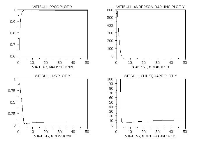
Program 2:
let gamma = 5.1
let y = weibull rand numb for i = 1 1 200
.
let gamma1 = 0.5
let gamma2 = 50
set ppcc plot axis points 449
.
multiplot corner coordinates 2 2 98 98
multiplot scale factor 2
multiplot 2 2
title automatic
title offset 2
justification center
height 1.7
tic mark offset units screen
ytic mark offset 3 0
.
weibull ppcc plot y
let shape = round(shape,1)
let maxppcc2 = round(maxppcc,3)
move 50 5
text Shape: ^shape, Max PPCC: ^maxppcc2
.
weibull anderson darling plot y
let shape = round(shape,1)
let minad2 = round(minad,3)
move 50 5
text Shape: ^shape, Min AD: ^minad2
.
weibull ks plot y
let shape = round(shape,1)
let minks = round(minks,3)
move 50 5
text Shape: ^shape, Min KS: ^minks
.
set chisquare limit 100
weibull chi-square plot y
let shape = round(shape,1)
let minchsq = round(minchisq,3)
move 50 5
text Shape: ^shape, Min Chi-Square: ^minchsq
.
end of multiplot
Date created: 08/30/2005 |
Last updated: 05/18/2023 Please email comments on this WWW page to [email protected]. | ||||||||||||||||||||||||