4. Process Modeling
4.6. Case Studies in Process Modeling
4.6.2. Alaska Pipeline

4.6.2.4.

Transformations to Improve Fit and Equalize Variances

Transformations

In regression modeling, we often apply transformations to achieve the following two goals:

1. to satisfy the homogeneity of variances assumption for the errors.
2. to linearize the fit as much as possible.

Some care and judgment is required in that these two goals can conflict. We generally try to achieve homogeneous variances first and then address the issue of trying to linearize the fit.

Plot of Common Transformations to Obtain Homogeneous Variances

The first step is to try transforming the response variable to find a tranformation that will equalize the variances. In practice, the square root, ln, and reciprocal transformations often work well for this purpose. We will try these first.

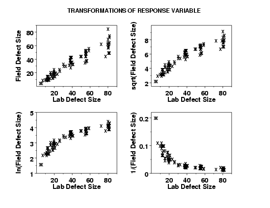
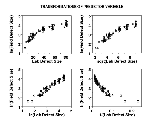
In examining these plots, we are looking for the plot that shows the most constant variability across the horizontal range of the plot.

This plot indicates that the ln transformation is a good candidate model for achieving the most homogeneous variances.

Plot of Common Transformations to Linearize the Fit

One problem with applying the above transformation is that the plot indicates that a straight-line fit will no longer be an adequate model for the data. We address this problem by attempting to find a transformation of the predictor variable that will result in the most linear fit. In practice, the square root, ln, and reciprocal transformations often work well for this purpose. We will try these first.

This plot shows that the ln transformation of the predictor variable is a good candidate model.

Box-Cox Linearity Plot

The previous step can be approached more formally by the use of the Box-Cox linearity plot. The α value on the x axis corresponding to the maximum correlation value on the y axis indicates the power transformation that yields the most linear fit.

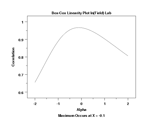
This plot indicates that a value of -0.1 achieves the most linear fit.

In practice, for ease of interpretation, we often prefer to use a common transformation, such as the ln or square root, rather than the value that yields the mathematical maximum. However, the Box-Cox linearity plot still indicates whether our choice is a reasonable one. That is, we might sacrifice a small amount of linearity in the fit to have a simpler model.

In this case, a value of 0.0 would indicate a ln transformation. Although the optimal value from the plot is -0.1, the plot indicates that any value between -0.2 and 0.2 will yield fairly similar results. For that reason, we choose to stick with the common ln transformation.

ln-ln Fit

Based on the above plots, we choose to fit a ln-ln model.

Parameter     Estimate    Stan. Dev    t Value
B0            0.281384      0.08093       3.48
B1            0.885175      0.02302      38.46
  
Residual standard deviation = 0.168260
Residual degrees of freedom = 105

Lack-of-fit F statistic              = 1.7032
Lack-of-fit critical value, F0.05,76,29 = 1.73

Note that although the residual standard deviation is significantly lower than it was for the original fit, we cannot compare them directly since the fits were performed on different scales.

Plot of Predicted Values

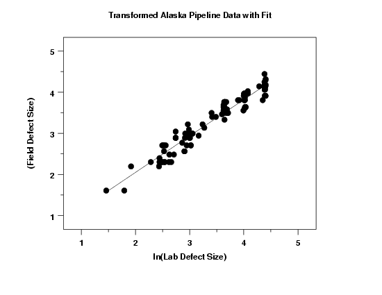
The plot of the predicted values with the transformed data indicates a good fit. In addition, the variability of the data across the horizontal range of the plot seems relatively constant.

6-Plot of Fit

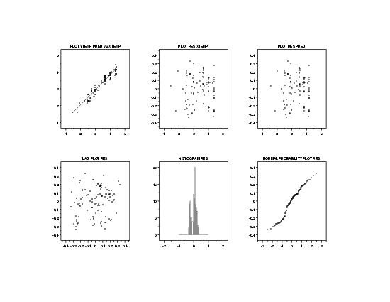
Since we transformed the data, we need to check that all of the regression assumptions are now valid.

The 6-plot of the residuals indicates that all of the regression assumptions are now satisfied.

Plot of Residuals

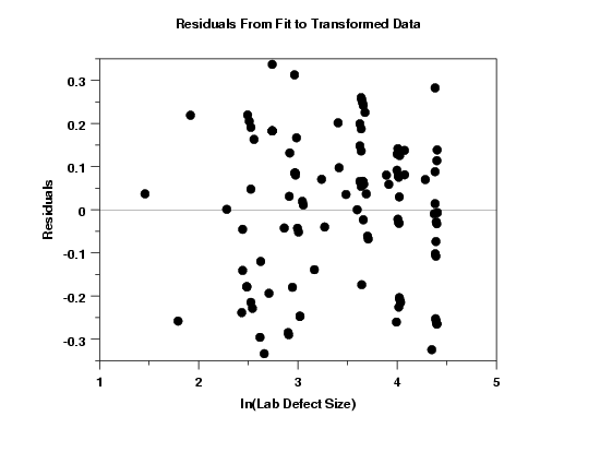
In order to see more detail, we generate a full-size plot of the residuals versus the predictor variable, as shown above. This plot suggests that the assumption of homogeneous variances is now met.