6. Process or Product Monitoring and Control
6.5. Tutorials

6.5.1.

What do we mean by "Normal" data?

The Normal distribution model

"Normal" data are data that are drawn (come from) a population that has a normal distribution. This distribution is inarguably the most important and the most frequently used distribution in both the theory and application of statistics. If \(X\) is a normal random variable, then the probability distribution of \(X\) is

Normal probability distribution

$$ f(x) = \frac{1}{\sigma \sqrt{2 \pi}} e^{ -\frac{1}{2} \left(\frac{x - \mu}{\sigma} \right)^2 } \,\,\,\,\,\, -\infty < x < \infty \, .$$

Parameters of normal distribution

The parameters of the normal distribution are the mean \(\mu\) and the standard deviation \(\sigma\) (or the variance \(\sigma^2\)). A special notation is employed to indicate that \(X\) is normally distributed with these parameters, namely $$ X \sim N(\mu, \, \sigma) \,\,\,\,\,\, \mbox{or} \,\,\,\,\,\, X \sim N(\mu, \, \sigma^2) \, . $$

Shape is symmetric and unimodal

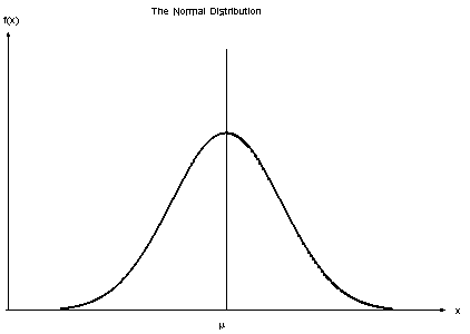
The shape of the normal distribution is symmetric and unimodal. It is called the bell-shaped or Gaussian distribution after its inventor, Gauss (although De Moivre also deserves credit).

The visual appearance is given below.

Property of probability distributions is that area under curve equals one

A property of a special class of non-negative functions, called probability distributions, is that the area under the curve equals unity. One finds the area under any portion of the curve by integrating the distribution between the specified limits. The area under the bell-shaped curve of the normal distribution can be shown to be equal to 1, and therefore the normal distribution is a probability distribution.

Interpretation of \(\sigma\)

There is a simple interpretation of \(\sigma\).

68.27 % of the population fall between \(\mu \pm 1 \sigma\)
95.45 % of the population fall between \(\mu \pm 2 \sigma\)
99.73 % of the population fall between \(\mu \pm 3 \sigma\)

The cumulative normal distribution

The cumulative normal distribution is defined as the probability that the normal variate is less than or equal to some value \(v\), or $$ P(X \le v) = F(v) = \int_{-\infty}^v \frac{1}{\sigma\sqrt{2\pi}} e^{ -\frac{1}{2} \left( \frac{x-\mu}{\sigma} \right)^2 } dx \, . $$ Unfortunately this integral cannot be evaluated in closed form and one has to resort to numerical methods. But even so, tables for all possible values of \(\mu\) and \(\sigma\) would be required. A change of variables rescues the situation. We let $$ z = \frac{x - \mu}{\sigma} \, . $$

Now the evaluation can be made independently of \(\mu\) and \(\sigma\); that is, $$ P(X \le v) = P \left(z \le \frac{v-\mu}{\sigma} \right) = \Phi \left( \frac{v-\mu}{\sigma} \right) \, , $$ where \(\Phi(.)\) is the cumulative distribution function of the standard normal distribution \((\mu=0, \, \sigma=1)\). $$ \phi(z) = \frac{1}{\sqrt{2 \pi}} e^{\frac{-z^2}{2}} $$

Tables for the cumulative standard normal distribution

Tables of the cumulative standard normal distribution are given in every statistics textbook and in the handbook. A rich variety of approximations can be found in the literature on numerical methods.

For example, if \(\mu = 0\) and \(\sigma=1\) then the area under the curve from \(\mu -1\sigma\) to \(\mu + 1 \sigma\) is the area from 0 - 1 to 0 + 1, which is 0.6827. Since most standard normal tables give area to the left of the lookup value, they will have for \(z = 1\) an area of 0.8413 and for \(z = -1\) an area of 0.1587. By subtraction we obtain the area between -1 and +1 to be 0.8413 - 0.1587 = 0.6826.