1. Exploratory Data Analysis
1.3. EDA Techniques
1.3.6. Probability Distributions
1.3.6.7. Tables for Probability Distributions

1.3.6.7.1.

Cumulative Distribution Function of the Standard Normal Distribution

How to Use This Table

The table below contains the area under the standard normal curve from 0 to z. This can be used to compute the cumulative distribution function values for the standard normal distribution.

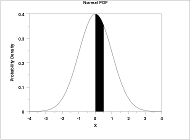
The table utilizes the symmetry of the normal distribution, so what in fact is given is

\( P[0 \le x \le |a|] \)

where a is the value of interest. This is demonstrated in the graph below for a = 0.5. The shaded area of the curve represents the probability that x is between 0 and a.

This can be clarified by a few simple examples.

1. What is the probability that x is less than or equal to 1.53? Look for 1.5 in the X column, go right to the 0.03 column to find the value 0.43699. Now add 0.5 (for the probability less than zero) to obtain the final result of 0.93699.

2. What is the probability that x is less than or equal to -1.53? For negative values, use the relationship

   \( P[x \le a] = 1 - P[x \le |a|] \;\;\;\;\; \mbox{for $x < 0$} \)

   From the first example, this gives 1 - 0.93699 = 0.06301.

3. What is the probability that x is between -1 and 0.5? Look up the values for 0.5 (0.5 + 0.19146 = 0.69146) and -1 (1 - (0.5 + 0.34134) = 0.15866). Then subtract the results (0.69146 - 0.15866) to obtain the result 0.5328.

To use this table with a non-standard normal distribution (either the location parameter is not 0 or the scale parameter is not 1), standardize your value by subtracting the mean and dividing the result by the standard deviation. Then look up the value for this standardized value.

A few particularly important numbers derived from the table below, specifically numbers that are commonly used in significance tests, are summarized in the following table:

p	0.001	0.005	0.010	0.025	0.050	0.100
Zp	-3.090	-2.576	-2.326	-1.960	-1.645	-1.282

p	0.999	0.995	0.990	0.975	0.950	0.900
Zp	+3.090	+2.576	+2.326	+1.960	+1.645	+1.282

These are critical values for the normal distribution.

Area under the Normal Curve from 0 to X X 0.00 0.01 0.02 0.03 0.04 0.05 0.06 0.07 0.08 0.09 0.0 0.00000 0.00399 0.00798 0.01197 0.01595 0.01994 0.02392 0.02790 0.03188 0.03586 0.1 0.03983 0.04380 0.04776 0.05172 0.05567 0.05962 0.06356 0.06749 0.07142 0.07535 0.2 0.07926 0.08317 0.08706 0.09095 0.09483 0.09871 0.10257 0.10642 0.11026 0.11409 0.3 0.11791 0.12172 0.12552 0.12930 0.13307 0.13683 0.14058 0.14431 0.14803 0.15173 0.4 0.15542 0.15910 0.16276 0.16640 0.17003 0.17364 0.17724 0.18082 0.18439 0.18793 0.5 0.19146 0.19497 0.19847 0.20194 0.20540 0.20884 0.21226 0.21566 0.21904 0.22240 0.6 0.22575 0.22907 0.23237 0.23565 0.23891 0.24215 0.24537 0.24857 0.25175 0.25490 0.7 0.25804 0.26115 0.26424 0.26730 0.27035 0.27337 0.27637 0.27935 0.28230 0.28524 0.8 0.28814 0.29103 0.29389 0.29673 0.29955 0.30234 0.30511 0.30785 0.31057 0.31327 0.9 0.31594 0.31859 0.32121 0.32381 0.32639 0.32894 0.33147 0.33398 0.33646 0.33891 1.0 0.34134 0.34375 0.34614 0.34849 0.35083 0.35314 0.35543 0.35769 0.35993 0.36214 1.1 0.36433 0.36650 0.36864 0.37076 0.37286 0.37493 0.37698 0.37900 0.38100 0.38298 1.2 0.38493 0.38686 0.38877 0.39065 0.39251 0.39435 0.39617 0.39796 0.39973 0.40147 1.3 0.40320 0.40490 0.40658 0.40824 0.40988 0.41149 0.41308 0.41466 0.41621 0.41774 1.4 0.41924 0.42073 0.42220 0.42364 0.42507 0.42647 0.42785 0.42922 0.43056 0.43189 1.5 0.43319 0.43448 0.43574 0.43699 0.43822 0.43943 0.44062 0.44179 0.44295 0.44408 1.6 0.44520 0.44630 0.44738 0.44845 0.44950 0.45053 0.45154 0.45254 0.45352 0.45449 1.7 0.45543 0.45637 0.45728 0.45818 0.45907 0.45994 0.46080 0.46164 0.46246 0.46327 1.8 0.46407 0.46485 0.46562 0.46638 0.46712 0.46784 0.46856 0.46926 0.46995 0.47062 1.9 0.47128 0.47193 0.47257 0.47320 0.47381 0.47441 0.47500 0.47558 0.47615 0.47670 2.0 0.47725 0.47778 0.47831 0.47882 0.47932 0.47982 0.48030 0.48077 0.48124 0.48169 2.1 0.48214 0.48257 0.48300 0.48341 0.48382 0.48422 0.48461 0.48500 0.48537 0.48574 2.2 0.48610 0.48645 0.48679 0.48713 0.48745 0.48778 0.48809 0.48840 0.48870 0.48899 2.3 0.48928 0.48956 0.48983 0.49010 0.49036 0.49061 0.49086 0.49111 0.49134 0.49158 2.4 0.49180 0.49202 0.49224 0.49245 0.49266 0.49286 0.49305 0.49324 0.49343 0.49361 2.5 0.49379 0.49396 0.49413 0.49430 0.49446 0.49461 0.49477 0.49492 0.49506 0.49520 2.6 0.49534 0.49547 0.49560 0.49573 0.49585 0.49598 0.49609 0.49621 0.49632 0.49643 2.7 0.49653 0.49664 0.49674 0.49683 0.49693 0.49702 0.49711 0.49720 0.49728 0.49736 2.8 0.49744 0.49752 0.49760 0.49767 0.49774 0.49781 0.49788 0.49795 0.49801 0.49807 2.9 0.49813 0.49819 0.49825 0.49831 0.49836 0.49841 0.49846 0.49851 0.49856 0.49861 3.0 0.49865 0.49869 0.49874 0.49878 0.49882 0.49886 0.49889 0.49893 0.49896 0.49900 3.1 0.49903 0.49906 0.49910 0.49913 0.49916 0.49918 0.49921 0.49924 0.49926 0.49929 3.2 0.49931 0.49934 0.49936 0.49938 0.49940 0.49942 0.49944 0.49946 0.49948 0.49950 3.3 0.49952 0.49953 0.49955 0.49957 0.49958 0.49960 0.49961 0.49962 0.49964 0.49965 3.4 0.49966 0.49968 0.49969 0.49970 0.49971 0.49972 0.49973 0.49974 0.49975 0.49976 3.5 0.49977 0.49978 0.49978 0.49979 0.49980 0.49981 0.49981 0.49982 0.49983 0.49983 3.6 0.49984 0.49985 0.49985 0.49986 0.49986 0.49987 0.49987 0.49988 0.49988 0.49989 3.7 0.49989 0.49990 0.49990 0.49990 0.49991 0.49991 0.49992 0.49992 0.49992 0.49992 3.8 0.49993 0.49993 0.49993 0.49994 0.49994 0.49994 0.49994 0.49995 0.49995 0.49995 3.9 0.49995 0.49995 0.49996 0.49996 0.49996 0.49996 0.49996 0.49996 0.49997 0.49997 4.0 0.49997 0.49997 0.49997 0.49997 0.49997 0.49997 0.49998 0.49998 0.49998 0.49998