8. Assessing Product Reliability
8.4. Reliability Data Analysis
8.4.1. How do you estimate life distribution parameters from censored data?

8.4.1.3.

A Weibull maximum likelihood estimation example

Reliability analysis using Weibull data

We will plot Weibull censored data and estimate parameters using data from a previous example (8.2.2.1).

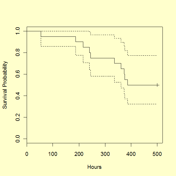
The recorded failure times were 54, 187, 216, 240, 244, 335, 361, 373, 375, and 386 hours, and 10 units that did not fail were removed from the test at 500 hours. The data are summarized in the following table.

    Time   Censored  Frequency
  54       0          1
 187       0          1
 216       0          1
 240       0          1
 244       0          1
 335       0          1
 361       0          1
 373       0          1
 375       0          1
 386       0          1
 500       1         10

The column labeled "Time" contains failure and censoring times, the "Censored" column contains a variable to indicate whether the time in column one is a failure time or a censoring time, and the "Frequency" column shows how many units failed or were censored at that time.

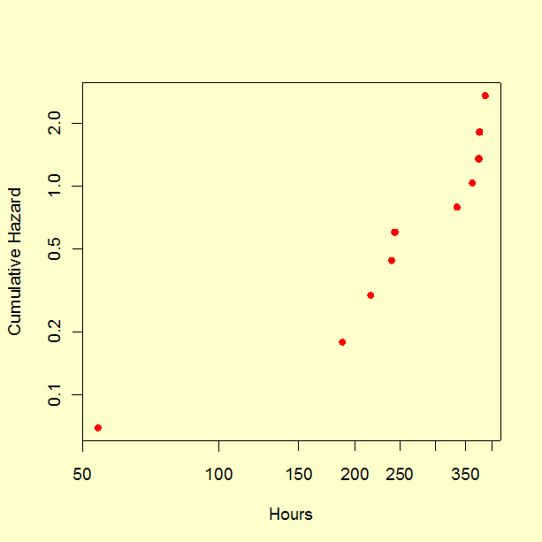
First, we generate a survival curve using the Kaplan-Meier method and a Weibull probability plot. Note: Some software packages might use the name "Product Limit Method" or "Product Limit Survival Estimates" instead of the equivalent name "Kaplan-Meier".

Next, we perform a regression analysis for a survival model assuming that failure times have a Weibull distribution. The Weibull characteristic life parameter (\(\eta\)) estimate is 606.5280 and the shape parameter (\(\beta\)) estimate is 1.7208.

The log-likelihood and Akaike's Information Criterion (AIC) from the model fit are -75.135 and 154.27. For comparison, we computed the AIC for the lognormal distribution and found that it was only slightly larger than the Weibull AIC.

Lognormal AIC   Weibull AIC 
    154.39         154.27

When comparing values of AIC, smaller is better. The probability density of the fitted Weibull distribution is shown below.

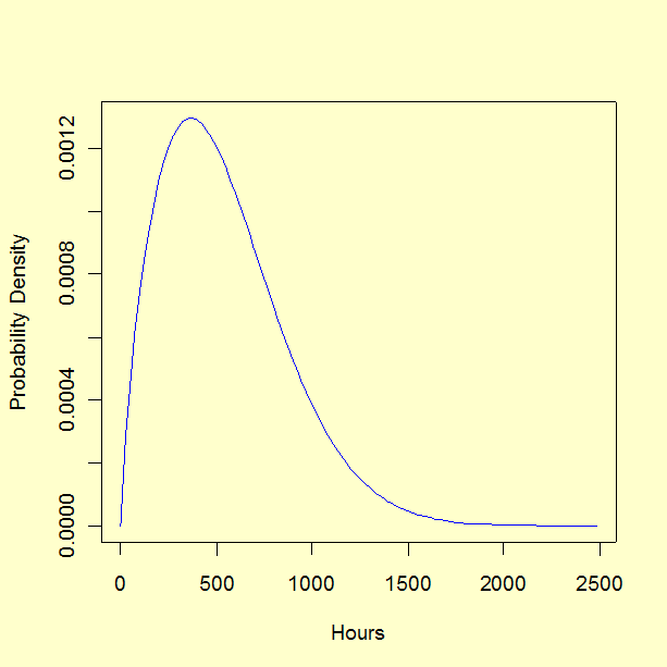
Based on the estimates of \(\eta\) and \(\beta\), the lifetime expected value and standard deviation are the following. $$ \begin{eqnarray} \hat{\eta} &=& 606.5280 \\ \\ \hat{\beta} &=& 1.7208 \\ \\ \hat{\mu} &=& \hat{\eta} \cdot \Gamma \left( 1 + 1/\hat{\beta} \right) = 540.737 \,\, \mbox{hours}\\ \\ \hat{\sigma} &=& \hat{\eta} \, \sqrt{\Gamma \left( 1+2/\hat{\beta} \right) - \left( \Gamma \left(1+1/\hat{\beta} \right) \right)^{2}} = 323.806 \,\, \mbox{hours} \end{eqnarray} $$ The greek letter, \(\Gamma\), represents the gamma function.

Discussion

Maximum likelihood estimation (MLE) is an accurate and easy way to estimate life distribution parameters, provided that a good software analysis package is available. The package should also calculate confidence bounds and log-likelihood values.

The analyses in this section can can be implemented using R code.