IGPPF

IGPPF (LET)

Library Function

Compute the inverse Gaussian percent point function with shape parameters gamma and mu.

The inverse Gaussian distribution has the following cumulative distribution function:

with and denoting the shape parameters and denoting the cumulative distribution function of the standard normal distribution.

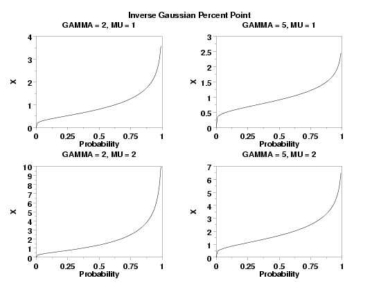
The percent point function is the inverse of the cumulative distribution function. The percent point function for the inverse Gaussian distribution does not exist in simple, closed form. It is computed by numerically inverting the inverse Gaussian cumulative distribution function using a bisection method.

The inverse Gaussian distribution can be generalized with location and scale parameters in the usual way.

LET <y> = IGPPF(<p>,<gamma>,<mu>,<loc>,<scale>)
                        <SUBSET/EXCEPT/FOR qualification>
where <p> is a variable or a parameter in the interval (0,1);
            <gamma> is number or parameter that specifies the first shape parameter;
            <mu> is number or parameter that specifies the second shape parameter;
            <loc> is number or parameter that specifies the location parameter;
            <scale> is number or parameter that specifies the scale parameter;
            <y> is a variable or a parameter (depending on what <x> is) where the computed inverse Gaussian ppf value is stored;
and where the <SUBSET/EXCEPT/FOR qualification> is optional.

Note that the location and scale parameters are optional.

LET A = IGPPF(0.95,2,1)
LET A = IGPPF(P1,2,1)
PLOT IGPPF(P,2,1.5) FOR P = 0 0.01 0.99

The case where = 1 is referred to as the Wald distribution. Enter HELP WALPDF for details.

None

None

IGCDF	= Compute the inverse Gaussian cumulative distribution function.
IGCHAZ	= Compute the inverse Gaussian cumulative hazard function.
IGHAZ	= Compute the inverse Gaussian hazard function.
IGPDF	= Compute the inverse Gaussian probability density function.
IGPPF	= Compute the inverse Gaussian percent point function.
CHSPDF	= Compute the chi-square probability density function.
FPDF	= Compute the F probability density function.
NORPDF	= Compute the normal probability density function.
TPDF	= Compute the t probability density function.
WEIPDF	= Compute the Weibull probability density function.
WALPDF	= Compute the Wald probability density function.
FLPDF	= Compute the fatigue life probability density function.
RIGPDF	= Compute the reciprocal inverse Gaussian probability density function.

"Continuous Univariate Distributions--Volume 1", Second Edition, Johnson, Kotz, and Balakrishnan, Wiley, 1994, chapter 15.

"Statistical Distributions", Third Edition, Evans, Hastings, and Peacock, Wiley, 2000, pp. 114-116.

Distributional Modeling

1990/5: Original implementation
2003/12: Modified to treat as a shape parameter instead of a location parameter.

 
X1LABEL Probability
Y1LABEL X
LABEL CASE ASIS
X1LABEL DISPLACEMENT 12
Y1LABEL DISPLACEMENT 12
MULTIPLOT SCALE FACTOR 2
MULTIPLOT 2 2
MULTIPLOT CORNER COORDINATES 0 0 100 95
TITLE GAMMA = 2, MU = 1
PLOT IGPPF(P,2,1) FOR P = 0  0.01  0.99
TITLE GAMMA = 5, MU = 1
PLOT IGPPF(P,5,1) FOR P = 0  0.01  0.99
TITLE GAMMA = 2, MU = 2
PLOT IGPPF(P,2,2) FOR P = 0  0.01  0.99
TITLE GAMMA = 5, MU = 2
PLOT IGPPF(P,5,2) FOR P = 0  0.01  0.99
END OF MULTIPLOT
JUSTIFICATION CENTER
MOVE 50 97
CASE ASIS
TEXT Inverse Gaussian Percent Point