SEASONAL LOWESS

SEASONAL LOWESS

Analysis Command

The SEASONAL LOWESS command decomposes a time series into trend, seasonal, and residual components using techniques based on locally weighted least squares. That is,
X(t) = TREND(t) + SEAS(t) + RES(t)

There are a number of time series techniques that are based on decomposing time series into a trend, seasonal, and residual component. The most popular of these is based on exponential smoothing. Seasonal lowess is a decomposition method based on locally weighted least squares.

In general, these methods are an alternative to autoregressive/moving average (ARMA) models. Decomposition methods are a preferrable approach when the trend and seasonal components dominate the series.

The seasonal and trend components are written to the file DPST1F.DAT (dpst1f.dat on Unix systems) and can be read back into Dataplot for further plotting and analysis. The internal variable RES contains the residual component and the internal variable PRED contains the trend plus the seasonality component. The sample program below demonstrates a common plot for displaying these components.

The SEASONAL LOWESS command accepts a number of options which can be defined by LET commands. The most important is the PERIOD parameter which identifies the number of seasons (e.g., 12 for monthly data). PERIOD defaults to 12. The STLWIDTH parameter identifies the number of data points to use in the LOWESS steps and defaults to N/10. It is similar to specifying the LOWESS FRACTION for standard LOWESS smoothing. The more points used, the more smoothing that occurs. The STLSDEG and STLTDEG parameters identify the polynomial degree used in the lowess for the seasonal and trend components respectively. By default, the seasonal lowess performs some robustness iterations. Enter

LET STLROBST = 1 to suppress this.

The mathematical details of this technique is described in

Cleveland, Cleveland, McRae, and Terpenning, "STL: A Seasonal-Trend Decomposition Procedure Based on Loess", Statistics Research Report, AT&T Bell Laboratories.

Dataplot uses the source code provided by these authors to implement the SEASONAL LOWESS command.

LET PERIOD = <value>
LET STLWIDTH = <value>
LET STLSDEG = <0/1/2>
LET STLTDEG = <0/1/2>
LET STLROBST = <0/1>
SEASONAL LOWESS <y> <SUBSET/EXCEPT/FOR qualification>
SKIP 0
READ DPST1F.DAT SEAS TREND
where <y> is the variable containing the raw data for which a seasonal lowess is to be performed;
and where the <SUBSET/EXCEPT/FOR qualification> is optional.

The LET commands are described in the Description section above. The READ DPST1F.DAT command is used to read the seasonal and trend components back into Dataplot.

LET PERIOD = 12
LET STLWIDTH = 24
LET STLSDEG = 1
LET STLTDEG = 1
LET STLROBST = 0
SEASONAL LOWESS Y

There is no default for the SEASONAL LOWESS command itself. The defaults for the various LET commands are given in the Description section.

SEASONAL LOESS is a synonym for SEASONAL LOWESS.

LOWESS SMOOTH	= Perform a lowess smooth.
ARMA	= Perform an ARMA fit.
FIT	= Carries out a least squares fit.

Cleveland, Cleveland, McRae, and Terpenning, "STL: A Seasonal-Trend Decomposition Procedure Based on Loess," Statistics Research Report, AT&T Bell Laboratories.

Cleveland, William S. (1993), "Visualizing Data," Hobart Press.

Robust Time Series Analysis

2000/1

skip 25
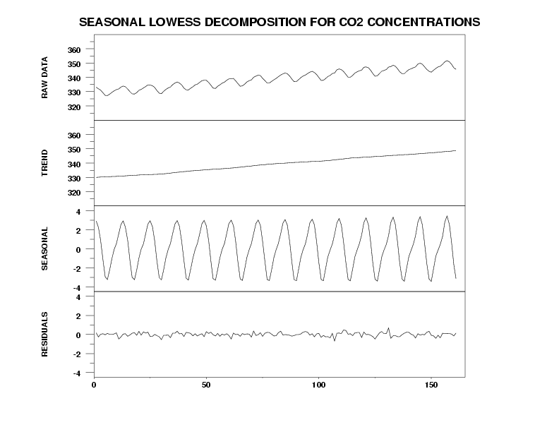
read mlco2mon.dat co2 date year month
.
. Perform Seasonal Lowess
.
let period = 12
let stlsdeg = 1
let stltdeg = 1
seasonal lowess co2
skip 0
read dpst1f.dat seas trend
.
. Generate plot
.
multiplot 4 1
multiplot scale factor 3
multiplot corner coordinates 0 10 100 95
frame corner coordinates 15 0 85 100
xlimits 0 150
tic offset units data
xtic offset 0 15
major xtic mark number 4
xtic marks off
xtic mark labels off
.
ylimits 320 360
major ytic mark number 5
ytic offser 10 10
y1label raw data
plot co2
y1label trend
plot trend
major ytic mark number 5
ylimits -4 4
ytic offser 0.5 0.5
y1label seasonal
plot seas
y1label residuals
x1tic marks on
x1tic mark labels on
plot res
end of multiplot
.
justification center
move 50 97
text SEASONAL LOWESS DECOMPOSITION FOR CO2 CONCENTRATIONS