EXTREME STUDENTIZED DEVIATE TEST
Name:
EXTREME STUDENTIZED DEVIATE TEST
Type:
Purpose:
Perform a generalized extreme studentized deviate (ESD) test for
outliers.
Description:
The generalized extreme Studentized deviate (ESD) test is used to
detect one or more outliers in a univariate data set that follows an
approximately normal distribution.
The primary limitation of the Grubbs test and the Tietjen-Moore test
is that the suspected number of outliers, k, must be specified
exactly. If k is not specified correctly, this can distort the
conclusions of these tests. On the other hand, the generalized ESD
test only requires that an upper bound for the suspected number of
outliers be specified.
Given the upper bound, r, the generalized ESD test essentially
performs r separate tests: a test for one outlier, a test for
two outliers, and so on up to r outliers.
The generalized ESD test is defined for the hypothesis:
|
H0:
|
There are no outliers in the data set
|
|
Ha:
|
There are up to r outliers in the data set
|
|
Test Statistic:
|
Compute
\( R_{1} = \mbox{max}_{i}|x_{i} - \bar{x}|/s \)
with
\( \bar{x} \) and s denoting the sample mean and sample
standard deviation, respectively.
Remove the observation that maximizes
\( |x_{i} - \bar{x}| \)
and then recompute the above statistic with n - 1
observations. Repeat this process until r observations
have been removed. This results in the r test
statistics R1, R2,
..., Rr.
|
|
Significance Level:
|
\( \alpha \)
|
|
Critical Region:
|
Corresponding to the r test statistics, compute
the following r critical values
\(
\lambda_{i} = \frac{t_{n-i-1,p(n-i)}}
{\sqrt{(n-i-1+t_{n-i-1,p}^{2}) (n-i+1)}}
\)
where i = 1, 2, ..., r,
\( t_{\nu,p} \)
is the 100p percentage point from the
t distribution with
\( \nu \) degrees of freedom and
\( p = 1 - \frac{\alpha}{2(n-i+1)} \).
The number of outliers is determined by finding the
largest i such that Ri >
\( \lambda_{i} \).
Simulation studies by Rosner indicate that this critical
value approximation is very accurate for n ≥ 25 and
reasonably accurate for n ≥ 15.
|
Note that although the generalized ESD is essentially Grubbs test
applied sequentially, there are a few important distinctions:
- The generalized ESD test makes approriate adjustments for the
critical values based on the number of outliers being tested
for that the sequential application of Grubbs test does not.
- If there is significant masking, applying Grubbs test
sequentially may stop too soon. The example below
identifies 3 outliers at the 5% level when using the
generalized ESD test. However, trying to use Grubbs test
sequentially would stop at the first iteration and
declare no outliers.
- Grubbs test allows one-sided tests (i.e., you can specify
a minimum test or the maximum test) in addition to two-sided
tests (both the minimum and the maximum value are tested).
The generalized ESD test is restricted to two-sided tests.
Syntax 1:
EXTREME STUDENTIZED DEVIATE TEST <y>
<SUBSET/EXCEPT/FOR qualification>
where <y> is the response variable being tested;
and where the <SUBSET/EXCEPT/FOR qualification> is optional.
Syntax 2:
EXTREME STUDENTIZED DEVIATE MULTIPLE TEST <y1> ... <yk>
<SUBSET/EXCEPT/FOR qualification>
where <y1> ... <yk> is a list of up to k response
variables;
and where the <SUBSET/EXCEPT/FOR qualification> is optional.
This syntax performs an extreme studentized deviate test on
<y1> then on <y2> and so on. Up to 30 response variables
can be specified.
Note that the syntax
EXTREME STUDENTIZED DEVIATE MULTIPLE TEST Y1 TO Y4
is supported. This is equivalent to
EXTREME STUDENTIZED DEVIATE MULTIPLE TEST Y1 Y2 Y3 Y4
Syntax 3:
EXTREME STUDENTIZED DEVIATE REPLICATED TEST <y> <x1>
... <xk>
<SUBSET/EXCEPT/FOR qualification>
where <y> is the response variable;
<x1> ... <xk> is a list of up to k group-id
variables;
and where the <SUBSET/EXCEPT/FOR qualification> is optional.
This syntax peforms a cross-tabulation of <x1> ... <xk>
and performs an extreme studentized deviate test for each unique
combination of cross-tabulated values. For example, if X1 has 3
levels and X2 has 2 levels, there will be a total of 6 extreme
studentized deviate tests performed.
Up to six group-id variables can be specified.
Note that the syntax
EXTREME STUDENTIZED DEVIATE REPLICATED TEST Y X1 TO X4
is supported. This is equivalent to
EXTREME STUDENTIZED DEVIATE REPLICATED TEST Y X1 X2 X3 X4
Examples:
EXTREME STUDENTIZED DEVIATE TEST Y1
EXTREME STUDENTIZED DEVIATE TEST Y1 LABID
EXTREME STUDENTIZED DEVIATE MULTIPLE TEST Y1 Y2 Y3
EXTREME STUDENTIZED DEVIATE REPLICATED TEST Y X1 X2
EXTREME STUDENTIZED DEVIATE TEST Y1 SUBSET TAG > 2
EXTREME STUDENTIZED DEVIATE MINIMUM TEST Y1
EXTREME STUDENTIZED DEVIATE MAXIMUM TEST Y1
Note:
The upper bound on the number of outliers to test for is specified
with the command
Note:
Masking and swamping are two issues that can affect outlier tests.
Masking can occur when we specify too few outliers in the test. For
example, if we are testing for a single outlier when there are in
fact two (or more) outliers, these additional outliers may influence
the value of the test statistic enough so that no points are
declared as outliers.
On the other hand, swamping can occur when we specify too many
outliers in the test. For example, if we are testing for two
outliers when there is in fact only a single outlier, both points
may be declared outliers.
The possibility of masking and swamping are an important reason
why it is useful to complement formal outlier tests with graphical
methods. Graphics can often help identify cases where masking or
swamping may be an issue.
Also, masking is one reason that trying to apply a single outlier
test sequentially can fail. If there are multiple outliers, masking
may cause the outlier test for the first outlier to return a
conclusion of no outliers (and so the testing for any additional
outliers is not done). Also, applying a single outlier test
sequentially does not properly adjust the critical value for the
overall test.
The masking/swamping issue explains the primary advantage of the
generalized ESD test. When there is masking or swamping, it is
not uncommon to see the conclusion for the prescence of outliers
change as the value for the number of outliers changes. By
weaking the assumption that the exact number of potential outliers
is known to the assumption that an upper bound is known (and we can
always pick this upper bound a little high if we do not have a good
handle on it), we are more likely to avoid distortions caused by
masking or swamping.
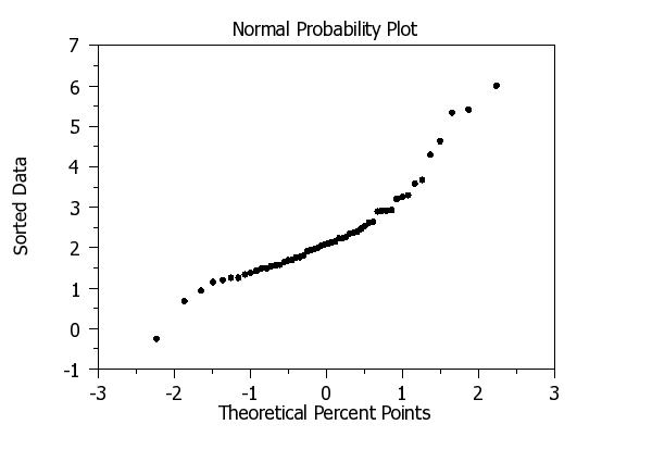
Note:
Tests for outliers are dependent on knowing the distribution of the
data. The generalized ESD test assumes that the data come from an
approximately normal distribution. For this reason, it is
strongly recommended that the extreme studentized deviate test be
complemented with a normal probability plot. If the data are not
approximately normally distributed, then the generalized ESD test
may be detecting the non-normality of the data rather than the
presence of outliers.
Note:
You can specify the number of digits in the generalized ESD output
with the command
SET WRITE DECIMALS <value>
Note:
The EXTREME STUDENTIZED DEVIATE TEST command automatically saves the
following parameters:
|
STATVAL
|
=
|
the value of the test statistic
|
|
PVAL
|
=
|
the p-value of the test statistic
|
|
CUTOFF0
|
=
|
the 0 percent point of the reference distribution
|
|
CUTOFF50
|
=
|
the 50 percent point of the reference distribution
|
|
CUTOFF75
|
=
|
the 75 percent point of the reference distribution
|
|
CUTOFF90
|
=
|
the 90 percent point of the reference distribution
|
|
CUTOFF95
|
=
|
the 95 percent point of the reference distribution
|
|
CUTOFF975
|
=
|
the 97.5 percent point of the reference distribution
|
|
CUTOFF99
|
=
|
the 99 percent point of the reference distribution
|
If the MULTIPLE or REPLICATED option is used, these values will
be written to the file "dpst1f.dat" instead.
Note:
In addition to the EXTREME STUDENTIZED DEVIATE TEST command, the
following command can also be used:
LET A = EXTREME STUDENTIZED DEVIATE Y
In addition to the above LET command, built-in statistics are
supported for 20+ different commands (enter
HELP STATISTICS
for details).
Default:
Synonyms:
ESD is a synonym for EXTREME STUDENTIZED DEVIATE
MULTIPLE ESD is a synonym for ESD MULTIPLE
REPLICATION ESD is a synonym for ESD REPLICATION
Related Commands:
References:
Rosner, Bernard (May 1983), "Percentage Points for a Generalized ESD
Many-Outlier Procedure," Technometrics, Vol. 25, No. 2,
pp. 165-172.
Iglewicz and Hoaglin (1993), "Volume 16: How to Detect and Handle
Outliers," The ASQC Basic Reference in Quality Control: Statistical
Techniques, Edward F. Mykytka, Ph.D., Editor.
Applications:
Implementation Date:
2009/11
2011/08: Fixed bug where the table for "Conclusions (2-Tailed Test)"
was printing the critical values in an inverted order
Program:
.  Step 1: Data from Rosner paper
.
serial read y
-0.25 0.68 0.94 1.15 1.20 1.26 1.26 1.34 1.38 1.43 1.49 1.49 1.55 1.56
 1.58 1.65 1.69 1.70 1.76 1.77 1.81 1.91 1.94 1.96 1.99 2.06 2.09 2.10
 2.14 2.15 2.23 2.24 2.26 2.35 2.37 2.40 2.47 2.54 2.62 2.64 2.90 2.92
 2.92 2.93 3.21 3.26 3.30 3.59 3.68 4.30 4.64 5.34 5.42 6.01
end of data
.
.  Step 2: Generate a normal probability plot
.
title case asis
title offset 2
label case asis
title Normal Probability Plot
y1label Sorted Data
x1label Theoretical Percent Points
char circle
char fill on
char hw 1.2 0.8
line blank
normal prob plot y
.
.  Step 3: Perform the generalized ESD outlier test
.
set write decimals 5
let noutlier = 10
extreme studentized deviate test y
The following output is generated.
            Generalized Extreme Studentized Deviate Test for
               Multiple Outliers (Assumption: Normality)

Response Variable: Y

Summary Statistics:
Number of Observations:                              54
Sample Minimum:                                -0.25000
Sample Maximum:                                 6.00999
Sample Mean:                                    2.32074
Sample SD:                                      1.18286


H0: There are no outliers
Ha: There is exactly     1 outlier
Potential Outlier Value Tested at This Step:              6.00999

Extreme Studentized Deviate Test Statistic Value:         3.11890

Percent Points of the Reference Distribution
-----------------------------------
  Percent Point               Value
-----------------------------------
            0.0    =          0.000
           50.0    =          2.532
           75.0    =          2.738
           90.0    =          2.987
           95.0    =          3.158
           97.5    =          3.318
           99.0    =          3.516

Conclusions (2-Tailed Test)
----------------------------------------------
  Alpha    CDF   Critical Value     Conclusion
----------------------------------------------
    10%    90%            2.987      Reject H0
     5%    95%            3.158      Accept H0
   2.5%  97.5%            3.318      Accept H0
     1%    99%            3.516      Accept H0


H0: There are no outliers
Ha: There are exactly     2 outliers
Potential Outlier Value Tested at This Step:              5.41999

Extreme Studentized Deviate Test Statistic Value:         2.94297

Percent Points of the Reference Distribution
-----------------------------------
  Percent Point               Value
-----------------------------------
            0.0    =          0.000
           50.0    =          2.524
           75.0    =          2.730
           90.0    =          2.980
           95.0    =          3.150
           97.5    =          3.311
           99.0    =          3.508

Conclusions (2-Tailed Test)
----------------------------------------------
  Alpha    CDF   Critical Value     Conclusion
----------------------------------------------
    10%    90%            2.980      Accept H0
     5%    95%            3.150      Accept H0
   2.5%  97.5%            3.311      Accept H0
     1%    99%            3.508      Accept H0


H0: There are no outliers
Ha: There are exactly     3 outliers
Potential Outlier Value Tested at This Step:              5.33999

Extreme Studentized Deviate Test Statistic Value:         3.17942

Percent Points of the Reference Distribution
-----------------------------------
  Percent Point               Value
-----------------------------------
            0.0    =          0.000
           50.0    =          2.516
           75.0    =          2.724
           90.0    =          2.972
           95.0    =          3.144
           97.5    =          3.303
           99.0    =          3.500

Conclusions (2-Tailed Test)
----------------------------------------------
  Alpha    CDF   Critical Value     Conclusion
----------------------------------------------
    10%    90%            2.972      Reject H0
     5%    95%            3.144      Reject H0
   2.5%  97.5%            3.303      Accept H0
     1%    99%            3.500      Accept H0


H0: There are no outliers
Ha: There are exactly     4 outliers
Potential Outlier Value Tested at This Step:              4.63999

Extreme Studentized Deviate Test Statistic Value:         2.81018

Percent Points of the Reference Distribution
-----------------------------------
  Percent Point               Value
-----------------------------------
            0.0    =          0.000
           50.0    =          2.509
           75.0    =          2.717
           90.0    =          2.964
           95.0    =          3.136
           97.5    =          3.295
           99.0    =          3.491

Conclusions (2-Tailed Test)
----------------------------------------------
  Alpha    CDF   Critical Value     Conclusion
----------------------------------------------
    10%    90%            2.964      Accept H0
     5%    95%            3.136      Accept H0
   2.5%  97.5%            3.295      Accept H0
     1%    99%            3.491      Accept H0


H0: There are no outliers
Ha: There are exactly     5 outliers
Potential Outlier Value Tested at This Step:             -0.25000

Extreme Studentized Deviate Test Statistic Value:         2.81557

Percent Points of the Reference Distribution
-----------------------------------
  Percent Point               Value
-----------------------------------
            0.0    =          0.000
           50.0    =          2.501
           75.0    =          2.709
           90.0    =          2.956
           95.0    =          3.128
           97.5    =          3.287
           99.0    =          3.482

Conclusions (2-Tailed Test)
----------------------------------------------
  Alpha    CDF   Critical Value     Conclusion
----------------------------------------------
    10%    90%            2.956      Accept H0
     5%    95%            3.128      Accept H0
   2.5%  97.5%            3.287      Accept H0
     1%    99%            3.482      Accept H0


H0: There are no outliers
Ha: There are exactly     6 outliers
Potential Outlier Value Tested at This Step:              4.29999

Extreme Studentized Deviate Test Statistic Value:         2.84817

Percent Points of the Reference Distribution
-----------------------------------
  Percent Point               Value
-----------------------------------
            0.0    =          0.000
           50.0    =          2.494
           75.0    =          2.701
           90.0    =          2.948
           95.0    =          3.120
           97.5    =          3.278
           99.0    =          3.474

Conclusions (2-Tailed Test)
----------------------------------------------
  Alpha    CDF   Critical Value     Conclusion
----------------------------------------------
    10%    90%            2.948      Accept H0
     5%    95%            3.120      Accept H0
   2.5%  97.5%            3.278      Accept H0
     1%    99%            3.474      Accept H0


H0: There are no outliers
Ha: There are exactly     7 outliers
Potential Outlier Value Tested at This Step:              3.67999

Extreme Studentized Deviate Test Statistic Value:         2.27932

Percent Points of the Reference Distribution
-----------------------------------
  Percent Point               Value
-----------------------------------
            0.0    =          0.000
           50.0    =          2.486
           75.0    =          2.693
           90.0    =          2.940
           95.0    =          3.112
           97.5    =          3.270
           99.0    =          3.463

Conclusions (2-Tailed Test)
----------------------------------------------
  Alpha    CDF   Critical Value     Conclusion
----------------------------------------------
    10%    90%            2.940      Accept H0
     5%    95%            3.112      Accept H0
   2.5%  97.5%            3.270      Accept H0
     1%    99%            3.463      Accept H0


H0: There are no outliers
Ha: There are exactly     8 outliers
Potential Outlier Value Tested at This Step:              3.58999

Extreme Studentized Deviate Test Statistic Value:         2.31036

Percent Points of the Reference Distribution
-----------------------------------
  Percent Point               Value
-----------------------------------
            0.0    =          0.000
           50.0    =          2.478
           75.0    =          2.685
           90.0    =          2.932
           95.0    =          3.103
           97.5    =          3.262
           99.0    =          3.455

Conclusions (2-Tailed Test)
----------------------------------------------
  Alpha    CDF   Critical Value     Conclusion
----------------------------------------------
    10%    90%            2.932      Accept H0
     5%    95%            3.103      Accept H0
   2.5%  97.5%            3.262      Accept H0
     1%    99%            3.455      Accept H0


H0: There are no outliers
Ha: There are exactly     9 outliers
Potential Outlier Value Tested at This Step:              0.68000

Extreme Studentized Deviate Test Statistic Value:         2.10158

Percent Points of the Reference Distribution
-----------------------------------
  Percent Point               Value
-----------------------------------
            0.0    =          0.000
           50.0    =          2.468
           75.0    =          2.677
           90.0    =          2.923
           95.0    =          3.093
           97.5    =          3.253
           99.0    =          3.444

Conclusions (2-Tailed Test)
----------------------------------------------
  Alpha    CDF   Critical Value     Conclusion
----------------------------------------------
    10%    90%            2.923      Accept H0
     5%    95%            3.093      Accept H0
   2.5%  97.5%            3.253      Accept H0
     1%    99%            3.444      Accept H0


H0: There are no outliers
Ha: There are exactly    10 outliers
Potential Outlier Value Tested at This Step:              3.29999

Extreme Studentized Deviate Test Statistic Value:         2.06717

Percent Points of the Reference Distribution
-----------------------------------
  Percent Point               Value
-----------------------------------
            0.0    =          0.000
           50.0    =          2.460
           75.0    =          2.668
           90.0    =          2.915
           95.0    =          3.084
           97.5    =          3.242
           99.0    =          3.435

Conclusions (2-Tailed Test)
----------------------------------------------
  Alpha    CDF   Critical Value     Conclusion
----------------------------------------------
    10%    90%            2.915      Accept H0
     5%    95%            3.084      Accept H0
   2.5%  97.5%            3.242      Accept H0
     1%    99%            3.435      Accept H0


Summary Table
----------------------------------------------------------------------
     Exact           Test       Critical       Critical       Critical
 Number of      Statistic          Value          Value          Value
  Outliers          Value            10%             5%             1%
----------------------------------------------------------------------
         1        3.11890        2.98680        3.15879        3.51571
         2        2.94297        2.97960        3.15142        3.50772
         3        3.17942        2.97224        3.14388        3.49952
         4        2.81018        2.96469        3.13616        3.49110
         5        2.81557        2.95697        3.12824        3.48246
         6        2.84817        2.94906        3.12012        3.47358
         7        2.27932        2.94094        3.11179        3.46445
         8        2.31036        2.93262        3.10324        3.45506
         9        2.10158        2.92408        3.09445        3.44539
        10        2.06717        2.91530        3.08542        3.43543
Date created: 09/09/2010
Last updated: 12/11/2023
Please email comments on this WWW page to
[email protected].
|
