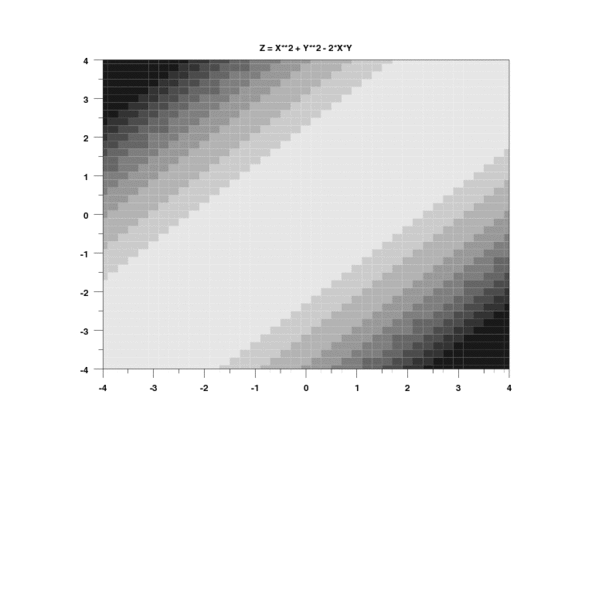
DISCRETE CONTOUR PLOT

DISCRETE CONTOUR PLOT

Graphics Command

Generates a discrete contour plot.

A contour plot is a graphical technique for representing a 3-dimensional z = f(x,y) surface by plotting constant-z "slices" (contours) on a 2-dimensional format. These slices are also referred to as iso-lines.

The discrete contour plot is a variation of the contour plot. Instead of drawing an isolines, a box is drawn at each square on the grid. The average response of the four points of this box is used to determine the level for that box. Levels are distinguished by the fill color of the box.

There is currently no "smoothing" of the color within the boxes to match neighboring boxes. If you want a smoother plot, then increase the number of points on the grid.

Both the levels and the colors to be used to identify the levels are set by the user.

The discrete contour plot is also referred to as a level plot or an image map.

DISCRETE CONTOUR PLOT <z> <x> <y> <z0>
                                    <SUBSET/EXCEPT/FOR qualification>
where <z> is the response (= dependent) variable;
            <x> is one horizontal axis variable;
            <y> is the other horizontal axis variable;
            <z0> is the variable of desired contour values;
and where the <SUBSET/EXCEPT/FOR qualification> is optional.

DISCRETE CONTOUR PLOT Z X Y Z0

The REGION COLOR, REGION PATTERN, and REGION BORDER COLOR commands are used to control the appearance of the plot. This is demonstrated in the sample program below.

Although you can use various types of region fill patterns, we typically just want solid-filled regions with the color denoting the level.

Unlike the standard contour plot, the discrete contour plot does not require equally spaced grids.

None

None

CONTOUR PLOT	= Generates a contour plot.
3D-PLOT	= Generates a 3-d data or function plot.
PLOT	= Generates a data or function plot.
REGION FILL COLOR	= Set the color for regions.

Unwin, Theus, and Hofmann (2006), "Graphics of Large Datasets: Visualizing a Million", Springer, pp. 49-50.

Analysis of Trivariate Data

2008/12

 
LET NTOT = 41*41
LET X = SEQUENCE -4 0.2 4 FOR I = 1 1 NTOT
LET Y = SEQUENCE -4 41 0.2 4
LET Z = X**2 + Y**2 - 2*X*Y
LET Z0 = SEQUENCE 5 5 40
. 
LIMITS -4.0  4.0
TIC MARK OFFSET 0 0
MAJOR TIC MARK NUMBER 9
MINOR TIC MARK NUMBER 1
REGION COLOR G90 G80 G70 G60 G50 G40 G30 G20 G10
.
TITLE OFFSET 2
TITLE X**2 + Y**2 - 2*X*Y
DISCRETE CONTOUR PLOT Z X Y Z0