BIVARIATE NORMAL TOLERANCE REGION PLOT

BIVARIATE NORMAL TOLERANCE REGION PLOT
BIVARIATE NORMAL CONFIDENCE REGION PLOT
POINCARE PLOT

Graphics Command

Generates a bivariate normal tolerance region plot. Alternatively, a bivariate normal confidence region plot or a Poincare plot can be generated.

The bivariate normal tolerance region and bivariate normal confidence region plots have a starting point of a Youden plot. The Poincare plot has as a starting point of a lag plot. All of these plots then overlay different types of ellipses on the basic underlying plot.

A tolerance interval calculate a confidence interval that contains at least a fixed percentage (or proportion) of the data.

There are two probability values involved in the tolerance region:

1. The coverage probability is the fixed percentage of the data to be covered. We call this \( \delta \).

2. The confidence level. We call this \( \gamma \).

That is, we can state with \( \gamma \)% confidence that at least (\ \delta; \)% of the data fall within the given limits. For example, if \( \gamma \) = 0.95 and \( \delta \) = 0.90, we say that we have a "95% confidence interval for 90% coverage".

The TOLERANCE LIMITS command is used to compute univariate normal tolerance intervals (it will also compute non-parametric tolerance interals). The BASIS TOLERANCE LIMITS is used to compute normal, lognormal, and Weibull tolerance limits.

The BIVARIATE NORMAL TOLERANCE REGION PLOT is used for the case where we have bivariate, normally distributed data. In this case, if X and Y denote our bivariate data, we define a region A such that

Pr(Pr[(X,Y) \( \varepsilon \) A] > \( \delta \)} = \( \gamma \)

Hall and Sheldon state that with a properly chosen K the following ellipse is the smallest region that will contain δ of the probability mass:

\( \frac{1}{1 - \rho^2} \left[ \left( \frac{x - \mu_x}{\sigma_x} \right) ^2 - 2 \rho \left( \frac{x - \mu_x}{\sigma_x} \right) \left( \frac{y - \mu_y}{\sigma_y} \right) + \left( \frac{y - \mu_y}{\sigma_y} \right) ^2 \right] = K \)

When we have a sample of n data points, we replace the population means, standard deviations, and correlation with the sample values in the above formula.

The problem then becomes how to find the appropriate value of K.

Hall and Sheldon describe how to find K for several different cases. We focus on their case 4 where the population means and standard deviations and the population correlation between X and Y are unknown.

Hall and Sheldon developed a table (Table 3 in their paper) using Monte Carlo methods for \( \gamma \) = 0.75, 0.90, and 0.95 and \( \delta \) = 0.50, 0.80, 0.90, and 0.95 for n = 10 to 50.

Dataplot will use the tabled values when appropriate. For n > 50 or for \( \gamma \) and \( \delta \) values not available in the table, Dataplot uses an approximation given on pp. 325-327 of Krishnamoorthy.

We recommend using the tabled values for \( \gamma \) and \( \delta \) for smaller values of n.

The BIVARIATE NORMAL TOLERANCE REGION PLOT generates a scatter plot of Y versus X and then overlays the tolerance region ellipse on this plot. Note that Dataplot allows multiple ellipses (corresponding to different values of \( \delta \)) to be overlaid on the plot.

You can specify the desired value of \( \gamma \) by entering the command

LET GAMMA = <value>

If you do not specify a value for \( \gamma \), then 0.95 will be used.

To specify a single value of \( \delta \), then enter the command

LET DELTA = <value>

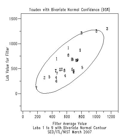
To specify multiple values of \( \delta \), see Syntax 3 below. If no \( \delta \) values are specified, then 0.90 will be used.

Alternatively, a bivariate normal confidence region plot can be generated. In this case, we are generating a joint confidence interval for the means of the two datasets. For this alternative, the ellipse has a similar form to the tolerance ellipse. However, the K is replaced with Hotelling's T²:

\( T^{2} = \frac{2(\rho - 1)}{\rho - 2} F_{(1 - \alpha),2,\rho - 1} \)

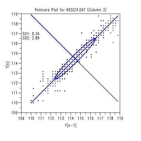
with F denoting the percent point function of the F distribution.

The bivariate normal confidence regions are discussed in the ISO 13528 standard based on the method given by Jackson.

The Poincare plots Y_i versus Y_i-1. This is equivalent to a lag plot. However, the Poincare plot adds an overlaid ellipse to the plot. Specifically, compute (where Y1 is Y_i and Y2 is Y_i-1 and Y is the original series)

\( X1 = \frac{Y1 - Y2}{\sqrt{2}} \)

\( X2 = \frac{Y1 + Y2}{\sqrt{2}} \)

X1 and X2 correspond to the rotation of Y1 and Y2 by \( \pi/4 \). Then the quantities SD1 and SD2 correspond to the standard deviations of X1 and X2, respectively. The quantities SD1 and SD2 and the ratio SD1/SD2 are used to characterize the original time series. Also, SD2 defines the radius of the major axis of the ellipse and SD1 defines the radius of the minor axis of the ellipse. The ellipse is centered at the means of Y1 and Y2.

The lag plot is typically used to detect first order autocorrelation (e.g., to test the independence of residuals in a regression model). The Poincare plot is typically used in a context where we expect first order autocorrelation and is used to characterize that autocorrelation.

BIVARIATE NORMAL TOLERANCE REGION PLOT <y1> <y2>
            <SUBSET/EXCEPT/FOR qualification>
where <y1> is the first response variable;
            <y2> is the second response variable;
and where the <SUBSET/EXCEPT/FOR qualification> is optional.

This syntax is used when there are no groups in the data and there is a single value of \( \delta \).

BIVARIATE NORMAL TOLERANCE REGION PLOT <y1> <y2> <lab>
            <SUBSET/EXCEPT/FOR qualification>
where <y1> is the first response variable;
            <y2> is the second response variable;
            <lab>is a group-id variable;
and where the <SUBSET/EXCEPT/FOR qualification> is optional.

This syntax is used when there are multiple groups in the data (e.g., multiple labs or multiple methods) and there is a single value of \( \delta \).

BIVARIATE NORMAL TOLERANCE REGION PLOT <y1> <y2> <lab> <delta>
                        <SUBSET/EXCEPT/FOR qualification>
where <y1> is the first response variable;
            <y2> is the second response variable;
            <lab> is a group-id variable;
            <delta> is a variable containing the desired values of delta;
and where the <SUBSET/EXCEPT/FOR qualification> is optional.

This syntax is used when there are multiple groups in the data (e.g., multiple labs or multiple methods) and multiple values of \( \delta \) are desired.

If you want multiple values of \( \delta \) when there are no groups, create a group-id variable with all values equal. For example

LET LAB = 1 FOR I = 1 1 N

BIVARIATE NORMAL CONFIDENCE REGION PLOT <y1> <y2>
            <SUBSET/EXCEPT/FOR qualification>
where <y1> is the first response variable;
            <y2> is the second response variable;
and where the <SUBSET/EXCEPT/FOR qualification> is optional.

This syntax is used when there are no groups in the data and there is a single value of \( \delta \) (here, \( \delta \) denotes confidence levels rather than coverage levels).

BIVARIATE NORMAL CONFIDENCE REGION PLOT <y1> <y2> <lab>
            <SUBSET/EXCEPT/FOR qualification>
where <y1> is the first response variable;
            <y2> is the second response variable;
            <lab>is a group-id variable;
and where the <SUBSET/EXCEPT/FOR qualification> is optional.

This syntax is used when there are multiple groups in the data (e.g., multiple labs or multiple methods) and there is a single value of \( \delta \) (here \( \delta \) denotes confidence levels rather than coverage levels).

BIVARIATE NORMAL CONFIDENCE REGION PLOT <y1> <y2> <lab> <delta>
                        <SUBSET/EXCEPT/FOR qualification>
where <y1> is the first response variable;
            <y2> is the second response variable;
            <lab> is a group-id variable;
            <delta> is a variable containing the desired values of delta;
and where the <SUBSET/EXCEPT/FOR qualification> is optional.

This syntax is used when there are multiple groups in the data (e.g., multiple labs or multiple methods) and multiple values of \( \delta \) (here \( \delta \) denotes confidence levels rather than coverage levels) are desired.

If you want multiple values of \( \delta \) when there are no groups, create a group-id variable with all values equal. For example

LET LAB = 1 FOR I = 1 1 N

POINCARE PLOT <y1>             <SUBSET/EXCEPT/FOR qualification>
where <y1> is the response variable;
and where the <SUBSET/EXCEPT/FOR qualification> is optional.

BIVARIATE NORMAL TOLERANCE REGION PLOT Y1 Y2
BIVARIATE NORMAL TOLERANCE REGION PLOT Y1 Y2 LAB
BIVARIATE NORMAL TOLERANCE REGION PLOT Y1 Y2 LAB DELTA
BIVARIATE NORMAL TOLERANCE REGION PLOT Y1 Y2 LAB ...
            SUBSET LAB > 2


BIVARIATE NORMAL CONFIDENCE REGION PLOT Y1 Y2
BIVARIATE NORMAL CONFIDENCE REGION PLOT Y1 Y2 LAB
BIVARIATE NORMAL CONFIDENCE REGION PLOT Y1 Y2 LAB DELTA
BIVARIATE NORMAL CONFIDENCE REGION PLOT Y1 Y2 LAB ...
            SUBSET LAB > 2


POINCARE PLOT Y1

You can use the CHARACTER and LINE commands to control the appearance of the plot. If there are NGROUP groups and NDELTA values of delta in the data, settings 1 through NDELTA control the appearance of the NDELTA ellipses and settings NDELTA + 1 through NDELTA + NGROUP control the appearance of the raw data for each group.

For the Poincare plot, the first setting controls the appearance of the ellipse, the second setting controls the appearance of the data points, the third setting controls the appearance of a line throught the major axis of the ellipse, and the fourth setting controls the appearance of a line through the minor axis of the ellipse. If you do not want the axis lines drawn, simply set the third and fourth LINE and CHARACTER settings to BLANK.

By default, the Poincare generates a lag 1 plot (i.e., Y_i versus Y_i-1). If you want a different lag, then enter
SET POINCARE PLOT LAG <value>

If <value> is less than 1 a lag 1 plot will be generated. If <value> is greater than N/4, this command will be ignored and a lag 1 plot will be generated.

The Poincare plot saves the following parameters

SD1	-	the radius of the minor axis of the ellipse
SD2	-	the radius of the major axis of the ellipse
SAREA	-	the area of the ellipse (= \( \pi \cdot \mbox{sd1} \cdot \mbox{sd2} \) )
CCM	-	the complex correlation measure

The CCM has been suggested as an alternative way to characterize the Poincare plot. It is defined by

\( CCM = \frac{1} {SAREA(N-1)} \sum_{i=1}^{N=2} {D} \)

where

D = (1/2)*determinant(A)

\( A = \left| \begin{array}{ccc} x1 & y1 & 1 \\ x2 & y2 & 1 \\ x3 & y3 & 1 \end{array} \right| \)

The (x1,y1), (x2,y2), and (x3,y3) define the coordinates of three successive points in the Poincare plot.

If any of the determinants have a condition number less than 1.0E-10, the CCM statistic will not be computed.

None

None

TOLERANCE LIMITS	= Generate normal or nonparameteric tolerance limits.
BASIS TOLERANCE LIMITS	= Generate normal, lognormal, and Weibull tolerance limits.
YOUDEN PLOT	= Generate a Youden plot.
LAG PLOT	= Generate a lag plot.
PLOT	= Generates a data or function plot.
CHARACTERS	= Sets the type for plot characters.
LINES	= Sets the type for plot lines.

Hall and Sheldon (1979), "Improved Bivariate Normal Tolerance Regions with Some Applications," Journal of Quality Technology, Vol. 11, No. 1, pp. 13-19.

Krishnamoorthy (2006), Handbook of Statistical Distributions with Applications, Chapman & Hall/CRC, pp. 325-327.

ISO 13528 (2005), "Statistical Methods for Use in Proficiency Testing by Interlaboratory Comparisons," ISO 13528:2005(E).

Jackson (1956), "Quality Control Methods for Two Related Variables," Industrial Quality Control, 7, pp. 2-6.

Tayel and AlSaba (2015), "Poincare Plot for Heart Rate Variability", International Journal of Medical, Health, Biomedical, Bioengineering and Pharmaceutical Engineering", Vol. 9, No. 9, pp. 708-711.

Interlaboratory Analysis

2007/04
2013/11: Support for BIVARIATE NORMAL CONFIDENCE REGION PLOT
2017/07: Support for POINCARE PLOT

 
ORIENTATION SQUARE
DIMENSION 20 COLUMNS
.
SKIP 25
READ STG.DAT LABID F LABAVE FAVE
.
TITLE OFFSET 2
TITLE CASE ASIS
LABEL CASE ASIS
TITLE Youden with Bivariate Normal Tolerance (95%-90%)
LET GAMMA = 0.95
LET DELTA = 0.90
X1LABEL Filter Average Value
Y1LABEL Lab Value for Filter
X2label Labs 1 to 9 with Bivariate Normal Contour
X3LABEL SED/ITL/NIST March 2007
.
TIC OFFSET UNITS DATA
XLIMITS 0 1200
XTIC OFFSET -25 100
YLIMITS 0 1500
YTIC OFFSET -350 100
.
CHARACTERS BLANK 1 2 3 4 5 6 7 8 9
LINES BLANK ALL
LINES SOLID
.
.  Base tolerance curve on all labs, but only plot first 9
.
BIVARIATE NORMAL TOLERANCE REGION PLOT LABAVE FAVE LABID
    

 
ORIENTATION SQUARE
DIMENSION 20 COLUMNS
.
SKIP 25
READ STG.DAT LABID F LABAVE FAVE
.
TITLE OFFSET 2
TITLE CASE ASIS
LABEL CASE ASIS
TITLE Youden with Bivariate Normal Confidence (95%)
LET DELTA = 0.95
X1LABEL Filter Average Value
Y1LABEL Lab Value for Filter
X2label Labs 1 to 9 with Bivariate Normal Contour
X3LABEL SED/ITL/NIST March 2007
.
TIC OFFSET UNITS DATA
XLIMITS 0 1200
XTIC OFFSET -25 100
YLIMITS 0 1500
YTIC OFFSET -350 100
.
CHARACTERS BLANK 1 2 3 4 5 6 7 8 9
LINES BLANK ALL
LINES SOLID
.
.  Base confidence curve on all labs, but only plot first 9
.
BIVARIATE NORMAL CONFIDENCE REGION PLOT LABAVE FAVE LABID
    

 
ORIENTATION SQUARE
DIMENSION 20 COLUMNS
.
READ NEGIZ4.DAT Y1 Y2 Y3 Y4
.
TITLE OFFSET 2
TITLE CASE ASIS
LABEL CASE ASIS
TITLE Poincare Plot for NEGIZ4.DAT (Column 3)
X1LABEL Y(n-1)
Y1LABEL Y(n)
.
CHARACTERS BLANK CIRCLE
CHARACTERS HW 0.5 0.375 ALL
CHARACTER FILL OFF ON
LINES SOLID BLANK DASH DASH
LINE THICKNESS 0.3 ALL
LINE COLOR BLUE ALL
.
POINCARE PLOT Y3
.
LET SD1 = ROUND(SD1,2)
LET SD2 = ROUND(SD2,2)
JUSTIFICATION LEFT
MOVE 16 75
TEXT SD1: ^SD1
MOVE 16 72
TEXT SD2: ^SD2