
|
|
BEST CPName:
There can be some variations in the above approaches. For example,
The choice of these critierion is complicated by the fact that adding additional variables will always increase the R2 of the fit (or at least not decrease it). However, including too many variables increases multicolinearity which results in numerically unstable models (i.e., you are essentially fitting noise). In addition, the model becomes more complex than it needs to be. A number of critierion have been proposed that attempt to balance maximizing the fit while trying to protect against overfitting. All subsets regression is the preferred algorithm in that it examines all models. However, it can be computationally impractical to perform all subsets regression when the number of independent variables becomes large. The primary disadvantage of forward/backward stepwise regression is that it may miss good candidate models. Also, they pick a single model rather than a list of good candidate models that can be examined closer. Dataplot addresses this issue with the BEST CP command. This is based on the following:
It should be emphasized that the BEST CP command is intended simply to identify good candidate models. Also, the BEST CP command uses a computationally fast algorithm that is not as accurate as the algorithm used by the FIT command. The FIT command should be applied to identified models that are of interest. Also, standard regression diagnostics should be examined to the candidate models of interest.
where <y> is the response (dependent) variable; <x1> .... <xk> is a list of one or more independent variables; and where the <SUBSET/EXCEPT/FOR qualification> is optional.
BEST CP Y X1 X2 X3 X4 X5 X6 X7 SUBSET TAG > 1
To change the number of candidate models chosen, enter the command
where <value> identifies the number of candidate models. Note that increasing <value> will result in greater time to generate the best candidate models. In most cases, the default value of 10 is adequate.
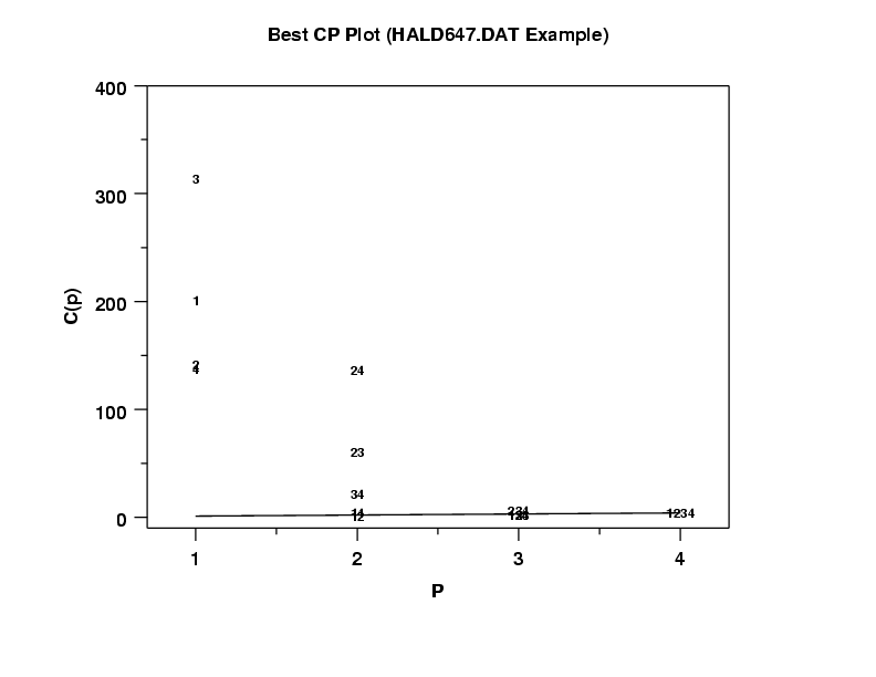
Dataplot writes the results of the CP analysis to file. The example program below shows how to generate a CP plot using these files. Specifically,
4
2
1
3
12
14
34
23
24
124
123
134
234
1234
Note:
Schwarz introduced an alternative information critierion called the Bayesian Information Critierion (BIC). The BIC penalizes the likelihood more than the AIC for additional parameters. For large n, the BIC can be approximated by
\(\hat{L}\) is the maximized value of the likelihood function. In the context of regression, the BIC can be computed as
where
The 2013/10 version of Dataplot added the BIC value for the selected models to the output. Note that the models are selected on the basis of Mallow's CP, not BIC. BIC is provided as an additional comparison.
C. L. Mallows (1966), "Choosing a Subset Regression," Joint Statistical Meetings, Los Angeles, CA. Sally Peavy, Shirley Bremer, Ruth Varner, and David Hogben (1986), "OMNITAB 80: An Interpretive System for Statistical and Numerical Data Analysis," NIST Special Publication 701. Thomas Ryan (1997), "Modern Regresion Methods," John Wiley, pp. 223-228. Schwarz (1978), "Estimating the dimension of a model," Annals of Statistics, Vol. 6, No. 2, pp. 461–464. Boisbunon, Canu, Fourdrinier, Strawderman, and Wells (2013), "AIC and Cp as estimators of loss for spherically symmetric distributions," arXiv:1308.2766.
2013/10: Reformatted output 2013/10: Added BIC values to output
skip 25
read hald647.dat y x1 x2 x3 x4
.
echo on
capture junk.dat
best cp y x1 x2 x3 x4
end of capture
.
skip 0
read dpst1f.dat p cp
read row labels dpst2f.dat
title case asis
label case asis
character rowlabels
line blank
tic offset units data
xtic offset 0.3 0.3
ytic offset 10 0
let maxp = maximum p
major xtic mark number maxp
xlimits 1 maxp
title Best CP Plot (HALD647.DAT Example)
x1label P
y1label C(p)
plot cp p
line solid
draw data 1 1 maxp maxp
The following output is generated for the BEST CP command.
            Regression with One Variable

---------------------------------------------
 C(p) Statistic            BIC      Variables
---------------------------------------------
      138.73082       59.98154              4
      142.48641       60.30789              2
      202.54876       64.64937              1
      315.15428       70.19729              3


            Regressions with   2 Variables

C(p) =        2.678, BIC =       27.115
---------------------------------------------
       Variable    Coefficient        F Ratio
---------------------------------------------
       X1              1.46831        146.522
       X2              0.66225        208.581


C(p) =        5.496, BIC =       30.437
---------------------------------------------
       Variable    Coefficient        F Ratio
---------------------------------------------
       X1              1.43995        108.224
       X4             -0.61395        159.294


C(p) =       22.373, BIC =       41.547
---------------------------------------------
       Variable    Coefficient        F Ratio
---------------------------------------------
       X3             -1.19985         40.295
       X4             -0.72460        100.356


C(p) =       62.438, BIC =       52.732
---------------------------------------------
       Variable    Coefficient        F Ratio
---------------------------------------------
       X2              0.73133         36.682
       X3             -1.00838         11.816


C(p) =      138.226, BIC =       62.324
---------------------------------------------
       Variable    Coefficient        F Ratio
---------------------------------------------
       X2              0.31090          0.172
       X4             -0.45694          0.431


---------------------------------------------
 C(p) Statistic            BIC      Variables
---------------------------------------------
      198.09465       66.81153           1  3


            Regressions with   3 Variables

C(p) =        3.018, BIC =       27.234
---------------------------------------------
       Variable    Coefficient        F Ratio
---------------------------------------------
       X1              1.45194        154.008
       X2              0.41611          5.025
       X4             -0.23654          1.863


C(p) =        3.041, BIC =       27.271
---------------------------------------------
       Variable    Coefficient        F Ratio
---------------------------------------------
       X1              1.69588         68.715
       X2              0.65691        220.546
       X3              0.25002          1.832


C(p) =        3.497, BIC =       27.987
---------------------------------------------
       Variable    Coefficient        F Ratio
---------------------------------------------
       X1              1.05184         22.112
       X3             -0.41004          4.235
       X4             -0.64280        208.240


C(p) =        7.337, BIC =       32.836
---------------------------------------------
       Variable    Coefficient        F Ratio
---------------------------------------------
       X2             -0.92342         12.426
       X3             -1.44797         96.939
       X4             -1.55704         41.654


            Regressions with   4 Variables

C(p) =        5.000, BIC =       29.769
---------------------------------------------
       Variable    Coefficient        F Ratio
---------------------------------------------
       X1              1.55109          4.336
       X2              0.51017          0.497
       X3              0.10191          0.018
       X4             -0.14406          0.041

         14 REGRESSIONS          56 OPERATIONS
The output can be displayed in graphical form.
Date created: 08/12/2003 |
Last updated: 12/11/2023 Please email comments on this WWW page to [email protected]. | |||||||||||||||||||||||||||||||||||