4.6. Case Studies in Process Modeling
4.6.4. Thermal Expansion of Copper Case Study
4.6.4.5. |
Cubic/Cubic Rational Function Model |
Based on the procedure described in 4.6.4.2, we fit the model: $$ y = A_0 + A_1 x + A_2 x^2 + A_3 x^3 - B_1 x - B_2 x^2 - B_3 x^3 + \varepsilon \, , $$ using the following seven representative points to generate the starting values for the C/C rational function.
 TEMP        THERMEXP
 ----        --------
  10             0
  30             2
  40             3
  50             5
 120            12
 200            15
 800            20
The coefficients from the preliminary linear fit of the seven points are:
A0 = -2.323648e+00
A1 =  3.530298e-01
A2 = -1.383334e-02
A3 =  1.766845e-04
B1 = -3.395949e-02
B2 =  1.100686e-04
B3 =  7.910518e-06
Parameter        Estimate    Stan. Dev    t Value
A0           1.07913        0.1710            6.3
A1          -0.122801       0.1203E-01      -10.2
A2           0.408837E-02   0.2252E-03       18.2
A3          -0.142848E-05   0.2610E-06       -5.5
B1          -0.576111E-02   0.2468E-03      -23.3
B2           0.240629E-03   0.1060E-04       23.0
B3          -0.123254E-06   0.1217E-07      -10.1

Residual standard deviation = 0.0818
Residual degrees of freedom = 229
The regression analysis yields the following estimated model. $$ \hat{y} = \frac{1.079 - 0.122x + 0.004097x^{2} - 0.00000143x^{3}} {1 - 0.00576x + 0.000241x^{2} - 0.000000123x^{3}} $$
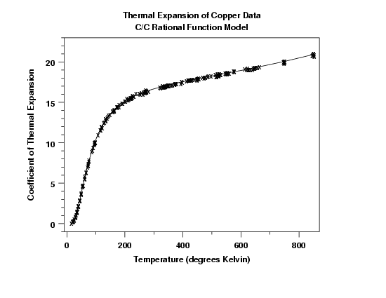
The fitted function with the raw data appears to show a reasonable fit.
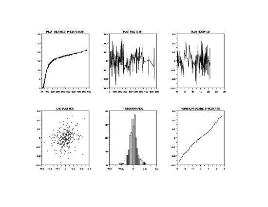
The 6-plot indicates no significant violation of the model assumptions. That is, the errors appear to have constant location and scale (from the residual plot in row 1, column 2), seem to be random (from the lag plot in row 2, column 1), and approximated well by a normal distribution (from the histogram and normal probability plots in row 2, columns 2 and 3).
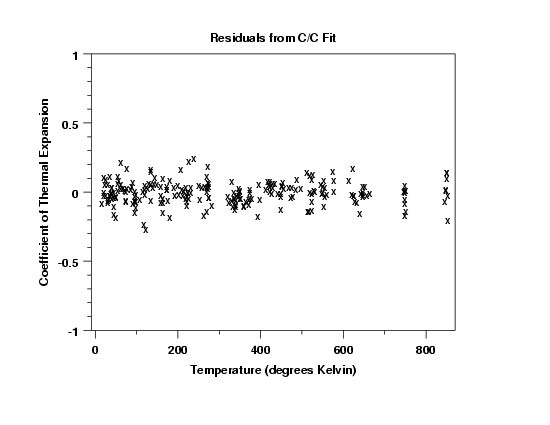
The full-sized residual plot suggests that the assumptions of constant location and scale for the errors are valid. No distinguishing pattern is evident in the residuals.


