4. Process Modeling
4.6. Case Studies in Process Modeling
4.6.4. Thermal Expansion of Copper Case Study

4.6.4.4.

Quadratic/Quadratic Rational Function Model

Q/Q Rational Function Model Starting Values

Based on the procedure described in 4.6.4.2, we fit the model: $$ y = A_0 + A_1 x + A_2 x^2 - B_1 x - B_2 x^2 + \varepsilon \, ,$$ using the following five representative points to generate the starting values for the Q/Q rational function.

Temp        THERMEXP
----        --------
 10             0
 50             5
120            12
200            15
800            20

The coefficients from the preliminary linear fit of the five points are:

A0 = -3.005450  
A1 =  0.368829 
A2 = -0.006828 
B1 = -0.011234 
B2 = -0.000306 

Nonlinear Fit Results

The results for the nonlinear fit are shown below.

Parameter        Estimate    Stan. Dev      t Value
A0             -8.028e+00    3.988e-01       -20.13   
A1              5.083e-01    1.930e-02        26.33   
A2             -7.307e-03    2.463e-04       -29.67   
B1             -7.040e-03    5.235e-04       -13.45   
B2             -3.288e-04    1.242e-05       -26.47   

Residual standard deviation = 0.5501
Residual degrees of freedom = 231

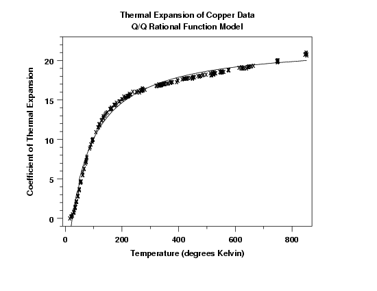
The regression yields the following estimated model. $$ \hat{y} = \frac{-8.028 + 0.508x - 0.007307x^{2}} {1 - 0.00704x - 0.0003288x^{2}} $$

Plot of Q/Q Rational Function Fit

We generate a plot of the fitted rational function model with the raw data.

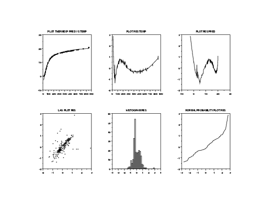
Looking at the fitted function with the raw data appears to show a reasonable fit.

6-Plot for Model Validation

Although the plot of the fitted function with the raw data appears to show a reasonable fit, we need to validate the model assumptions. The 6-plot is an effective tool for this purpose.

The plot of the residuals versus the predictor variable temperature (row 1, column 2) and of the residuals versus the predicted values (row 1, column 3) indicate a distinct pattern in the residuals. This suggests that the assumption of random errors is badly violated.

Residual Plot

We generate a full-sized residual plot in order to show more detail.

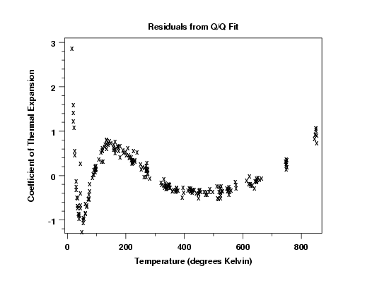
The full-sized residual plot clearly shows the distinct pattern in the residuals. When residuals exhibit a clear pattern, the corresponding errors are probably not random.