4. Process Modeling
4.6. Case Studies in Process Modeling
4.6.3. Ultrasonic Reference Block Study

4.6.3.4.

Weighting to Improve Fit

Weighting

Another approach when the assumption of constant variance of the errors is violated is to perform a weighted fit. In a weighted fit, we give less weight to the less precise measurements and more weight to more precise measurements when estimating the unknown parameters in the model.

Finding an Appropriate Weight Function

Techniques for determining an appropriate weight function were discussed in detail in Section 4.4.5.2.

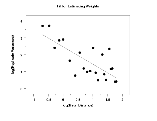
In this case, we have replication in the data, so we can fit the power model $$ \begin{eqnarray} \ln{(\hat{\sigma}_i^2)} & = & \ln{(\gamma_1x_i^{\gamma_2})} \\ & & \\ & = & \ln{(\gamma_1)} + \gamma_2\ln{(x_i}) \end{eqnarray} $$ to the variances from each set of replicates in the data and use $$ w_i = \frac{1}{x^{\hat{\gamma}_2}_i} $$ for the weights.

Fit for Estimating Weights

The following results were obtained for the fit of ln(variances) against ln(means) for the replicate groups.

Parameter       Estimate    Stan. Dev    t Value
γ0                2.5369       0.1919       13.1
γ1               -1.1128       0.1741       -6.4

Residual standard deviation = 0.6099
Residual degrees of freedom = 20

The fit output and plot from the replicate variances against the replicate means shows that the linear fit provides a reasonable fit, with an estimated slope of -1.1128.

Based on this fit, we used an estimate of -1.0 for the exponent in the weighting function.

Residual Plot for Weight Function

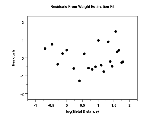
The residual plot from the fit to determine an appropriate weighting function reveals no obvious problems.

Numerical Results from Weighted Fit

The results of the weighted fit are shown below.

Parameter       Estimate    Stan. Dev    t Value
b1              0.146999   0.1505E-01        9.8
b2              0.005280   0.4021E-03       13.1
b3              0.012388   0.7362E-03       16.8

Residual standard deviation = 4.11
Residual degrees of freedom = 211

Plot of Predicted Values

To assess the quality of the weighted fit, we first generate a plot of the predicted line with the original data.

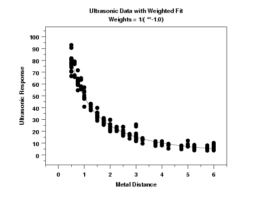
The plot of the predicted values with the data indicates a good fit. The model for the weighted fit is $$ \hat{y} = \frac{\exp(-0.147x)}{0.00528 + 0.0124x} $$

6-Plot of Fit

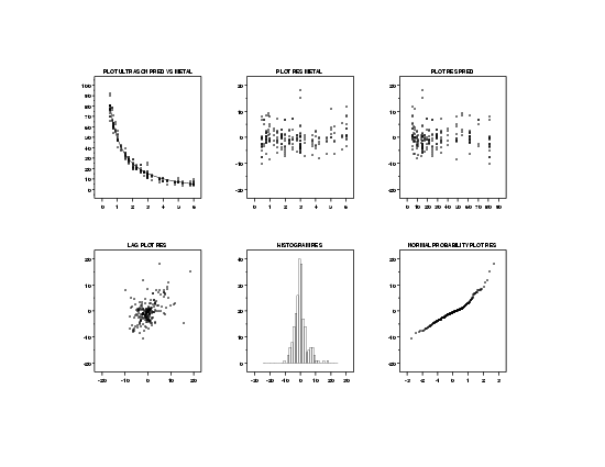
We need to verify that the weighted fit does not violate the regression assumptions. The 6-plot indicates that the regression assumptions are satisfied.

Plot of Residuals

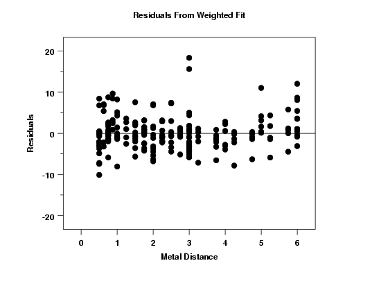
In order to check the assumption of equal error variances in more detail, we generate a full-sized version of the residuals versus the predictor variable. This plot suggests that the residuals now have approximately equal variability.