6. Process or Product Monitoring and Control
6.4. Introduction to Time Series Analysis
6.4.5. Multivariate Time Series Models

6.4.5.1.

Example of Multivariate Time Series Analysis

Bivariate Gas Furance Example

The gas furnace data from Box, Jenkins, and Reinsel, 1994 is used to illustrate the analysis of a bivariate time series. Inside the gas furnace, air and methane were combined in order to obtain a mixture of gases containing CO\(_2\) (carbon dioxide). The input series \(x_t\) is the methane gas feedrate and the CO\(_2\) concentration is the output series \(y_t\).

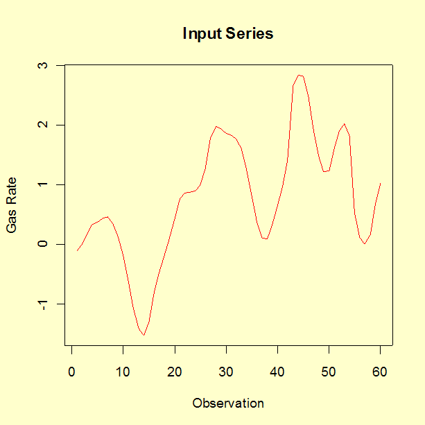
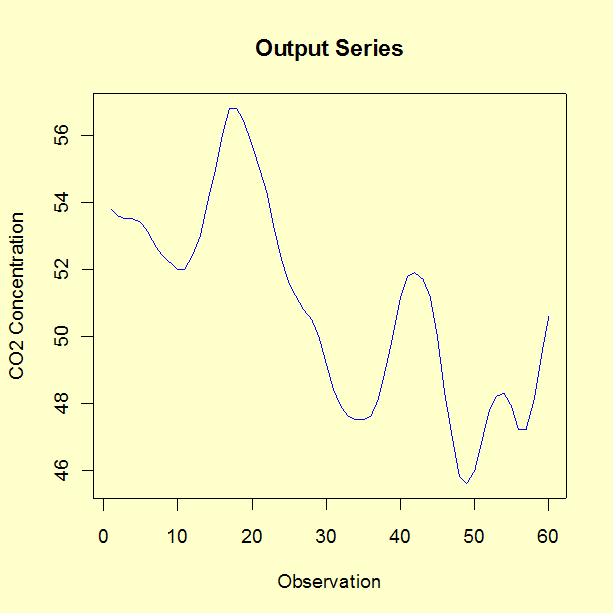
In this experiment 296 successive pairs of observations \((x_t, \, y_t)\) were collected from continuous records at 9-second intervals. For the analysis described here, only the first 60 pairs were used. We fit an ARV(2) model as described in 6.4.5. This data set is available as a text file.

Plots of input and output series

The plots of the input and output series are displayed below. 

Model Fitting

The scalar form of the ARV(2) model is the following. $$ \begin{eqnarray} x_t & = & \phi_{1.11}x_{t-1} + \phi_{2.11}x_{t-2} + \phi_{1.12}y_{t-1} + \phi_{2.12}y_{t-2} + a_{1t} \\ & & \\ y_t & = & \phi_{1.22}y_{t-1} + \phi_{2.22}y_{t-2} + \phi_{1.21}x_{t-1} + \phi_{2.21}x_{t-2} + a_{2t} \end{eqnarray} $$ The equation for \(x_t\) corresponds to gas rate while the equation for \(y_t\) corresponds to CO\(_2\) concentration.

The parameter estimates for the equation associated with gas rate are the following.

         Estimate  Std. Err.  t value   Pr(>|t|)  
a1t       0.003063   0.035769    0.086      0.932    
φ1.11     1.683225   0.123128   13.671    < 2e-16
φ2.11    -0.860205   0.165886   -5.186   3.44e-06
φ1.12    -0.076224   0.096947   -0.786      0.435    
φ2.12     0.044774   0.082285    0.544      0.589    

Residual standard error:  0.2654 based on 53 degrees of freedom
Multiple R-Squared:  0.9387
Adjusted R-squared:  0.9341 
F-statistic:  203.1 based on 4 and 53 degrees of freedom  
p-value:  < 2.2e-16 

The parameter estimates for the equation associated with CO\(_2\) concentration are the following.

        Estimate  Std. Err.  t value   Pr(>|t|) 
a2t      -0.03372    0.01615   -2.088   0.041641   
φ1.22     1.22630    0.04378   28.013    < 2e-16
φ2.22    -0.40927    0.03716  -11.015   2.57e-15
φ1.21     0.22898    0.05560    4.118   0.000134
φ2.21    -0.80532    0.07491  -10.751   6.29e-15

Residual standard error:  0.1198 based on 53 degrees of freedom
Multiple R-Squared:  0.9985     
Adjusted R-squared:  0.9984 
F-statistic:  8978 based on 4 and 53 degrees of freedom
p-value:  < 2.2e-16 

Box-Ljung tests performed for each series to test the randomness of the first 24 residuals were not significant. The \(p\)-values for the tests using CO\(_2\) concentration residuals and gas rate residuals were 0.4 and 0.6, respectively.

Forecasting

The forecasting method is an extension of the model and follows the theory outlined in the previous section. The forecasted values of the next six observations (61-66) and the associated 90 % confidence limits are shown below for each series.

             90% Lower   Concentration   90% Upper
Observation    Limit       Forecast        Limit
-----------  ---------     --------      ---------
    61          51.0         51.2           51.4
    62          51.0         51.3           51.6
    63          50.6         51.0           51.4
    64          49.8         50.5           51.1
    65          48.7         50.0           51.3
    66          47.6         49.7           51.8


             90% Lower     Rate     90% Upper
Observation    Limit     Forecast     Limit
-----------  ---------   --------   ---------
    61         0.795       1.231      1.668
    62         0.439       1.295      2.150
    63         0.032       1.242      2.452
    64        -0.332       1.128      2.588
    65        -0.605       1.005      2.614
    66        -0.776       0.908      2.593