6. Process or Product Monitoring and Control
6.4. Introduction to Time Series Analysis
6.4.4. Univariate Time Series Models

6.4.4.9.

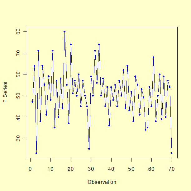
Example of Univariate Box-Jenkins Analysis

Series F

We analyze the series F data set in Box, Jenkins, and Reinsel, 1994. A plot of the 70 raw data points is shown below. The data do not appear to have a seasonal component or a noticeable trend. (The stationarity of the series was verified by fitting a straight line to the data versus time period. The slope was not found to be significantly different from zero (\(p\)-value = 0.2).)

Model Identification

We compute the autocorrelation function (ACF) of the data for the first 35 lags to determine the type of model to fit to the data. We list the numeric results and plot the ACF (along with 95 % confidence limits) versus the lag number.

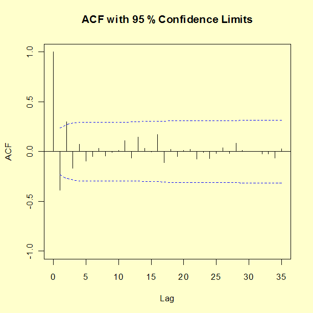
 Lag          ACF
   0  1.000000000
   1 -0.389878319
   2  0.304394082
   3 -0.165554717
   4  0.070719321
   5 -0.097039288
   6 -0.047057692
   7  0.035373112
   8 -0.043458199
   9 -0.004796162
  10  0.014393137
  11  0.109917200
  12 -0.068778492
  13  0.148034489
  14  0.035768581
  15 -0.006677806
  16  0.173004275
  17 -0.111342583
  18  0.019970791
  19 -0.047349722
  20  0.016136806
  21  0.022279561
  22 -0.078710582
  23 -0.009577413
  24 -0.073114034
  25 -0.019503289
  26  0.041465024
  27 -0.022134370
  28  0.088887299
  29  0.016247148
  30  0.003946351
  31  0.004584069
  32 -0.024782198
  33 -0.025905040
  34 -0.062879966
  35  0.026101117

The ACF values alternate in sign and decay quickly after lag 2, indicating that an AR(2) model is appropriate for the data.

Model Fitting

We fit an AR(2) model to the data. $$ X_t = \delta + \phi_1 X_{t-1} + \phi_2 X_{t-2} + A_t $$ The model fitting results are shown below.

Source  Estimate  Standard Error
------  --------  --------------
φ1       -0.3198      0.1202
φ2        0.1797      0.1202

δ = 51.1286 
Residual standard deviation = 10.9599

Test randomness of residuals:
Standardized Runs Statistic Z = 0.4887, p-value = 0.625

Forecasting

Using our AR(2) model, we forcast values six time periods into the future.

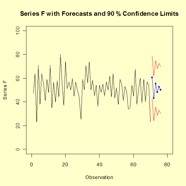
Period  Prediction   Standard Error
  71      60.6405       10.9479
  72      43.0317       11.4941
  73      55.4274       11.9015
  74      48.2987       12.0108
  75      52.8061       12.0585
  76      50.0835       12.0751

The "historical" data and forecasted values (with 90 % confidence limits) are shown in the graph below.