6.4. Introduction to Time Series Analysis
6.4.4. Univariate Time Series Models
6.4.4.6. Box-Jenkins Model Identification
6.4.4.6.1. |
Model Identification for Southern Oscillations Data |
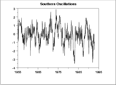
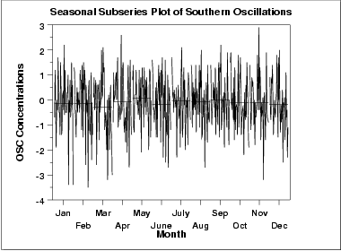
The first example is for the southern oscillations data set. We start with the run sequence plot and seasonal subseries plot to determine if we need to address stationarity and seasonality.

The run sequence plot indicates stationarity.

The seasonal subseries plot indicates that there is no significant seasonality.
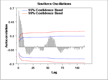
Since the above plots show that this series does not exhibit any significant non-stationarity or seasonality, we generate the autocorrelation and partial autocorrelation plots of the raw data.

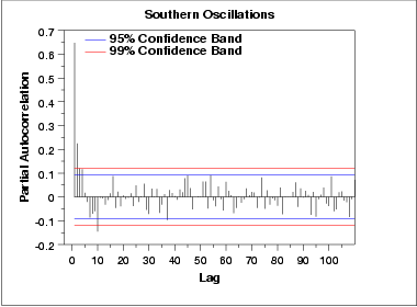
The autocorrelation plot shows a mixture of exponentially decaying and damped sinusoidal components. This indicates that an autoregressive model, with order greater than one, may be appropriate for these data. The partial autocorrelation plot should be examined to determine the order.

The partial autocorrelation plot suggests that an AR(2) model might be appropriate.
In summary, our intial attempt would be to fit an AR(2) model with no seasonal terms and no differencing or trend removal. Model validation should be performed before accepting this as a final model.

