6.4.3.6. Example of Triple Exponential Smoothing

6. Process or Product Monitoring and Control
6.4. Introduction to Time Series Analysis
6.4.3. What is Exponential Smoothing?

6.4.3.6. Example of Triple Exponential Smoothing

Example comparing single, double, triple exponential smoothing

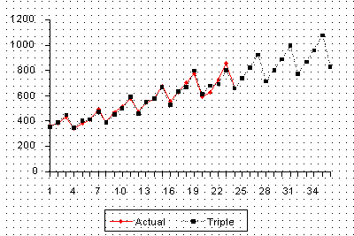
This example shows comparison of single, double and triple exponential smoothing for a data set.

The following data set represents 24 observations. These are six years of quarterly data (each year has four quarters).

Table showing the data for the example

	Quarter	Period	Sales		Quarter	Period	Sales

90	1	1	362	93	1	13	544
	2	2	385		2	14	582
	3	3	432		3	15	681
	4	4	341		4	16	557
91	1	5	382	94	1	17	628
	2	6	409		2	18	707
	3	7	498		3	19	773
	4	8	387		4	20	592
92	1	9	473	95	1	21	627
	2	10	513		2	22	725
	3	11	582		3	23	854
	4	12	474		4	24	661

The reader can download the data as a text file.

Plot of raw data with single, double, and triple exponential forecasts

Plot of raw data with triple exponential forecasts

Actual Time Series with forecasts

Plot of raw data with triple exponential forecasts

Comparison of MSEs

**Comparison of MSEs**
MSE	$\alpha$ demand	$\gamma$ trend	$\beta$ seasonality

6906	0.4694
5054	0.1086	1.0000
936	1.0000		1.0000
520	0.7556	0.0000	0.9837

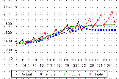
The updating coefficients were chosen by a computer program such that the MSE for each of the methods was minimized.

Example of the computation of the Initial Trend

Computation of initial trend

The data set consists of quarterly sales data. The season is 1 year and since there are 4 quarters per year, $L=4$. Using the formula we obtain: $$ \begin{eqnarray} b_1 & = & \frac{1}{4} \left[ \left( \frac{y5-y1}{4} \right) + \left( \frac{y6-y2}{4} \right) + \left( \frac{y7-y3}{4} \right) + \left( \frac{y8-y4}{4} \right) \right] \\ & & \\ & & \\ & = & \frac{1}{4} \left[ \left( \frac{382-362}{4} \right) + \left( \frac{409-385}{4} \right) + \left( \frac{498-432}{4} \right) + \left( \frac{387-341}{4} \right) \right] \\ & & \\ & & \\ & = & \frac{5 + 6 + 16.5 + 11.5}{4} = 9.75 \, . \end{eqnarray} $$

Example of the computation of the Initial Seasonal Indices

Table of initial seasonal indices

	1	2	3	4	5	6

1	362	382	473	544	628	627
2	385	409	513	582	707	725
3	432	498	582	681	773	854
4	341	387	474	557	592	661

$\bar{X}$	380	419	510.5	591	675	716.75

In this example we used the full 6 years of data. Other schemes may use only 3, or some other number of years. There are also a number of ways to compute initial estimates.