6. Process or Product Monitoring and Control
6.4. Introduction to Time Series Analysis
6.4.3. What is Exponential Smoothing?

6.4.3.4.

Forecasting with Double Exponential Smoothing(LASP)

Forecasting formula

The one-period-ahead forecast is given by: $$F_{t+1}=S_t+b_t.$$

The $m$-periods-ahead forecast is given by: $$F_{t+m}=S_t+m{b}_t.$$

Example

Example

Consider once more the data set:

6.4,  5.6,  7.8,  8.8,  11,  11.6,  16.7,  15.3,  21.6,  22.4.

Now we will fit a double smoothing model with $\alpha =0.3623$ and $\gamma =1.0$. These are the estimates that result in the lowest possible MSE when comparing the orignal series to one step ahead at a time forecasts (since this version of double exponential smoothing uses the current series value to calculate a smoothed value, the smoothed series cannot be used to determine an $\alpha$ with minimum MSE). The chosen starting values are $S_1=y_1=6.4$ and $b_1=((y_2-y_1)+(y_3-y_2)+(y_4-y_3))/3=0.8$.

For comparison's sake we also fit a single smoothing model with $\alpha =0.977$ (this results in the lowest MSE for single exponential smoothing).

The MSE for double smoothing is 3.7024.
The MSE for single smoothing is 8.8867.

Forecasting results for the example

The smoothed results for the example are:

Data	Double	Single
6.4	6.4
5.6	6.6 (Forecast = 7.2)	6.4
7.8	7.2 (Forecast = 6.8)	5.6
8.8	8.1 (Forecast = 7.8)	7.8
11.0	9.8 (Forecast = 9.1)	8.8
11.6	11.5 (Forecast = 11.4)	10.9
16.7	14.5 (Forecast = 13.2)	11.6
15.3	16.7 (Forecast = 17.4)	16.6
21.6	19.9 (Forecast = 18.9)	15.3
22.4	22.8 (Forecast = 23.1)	21.5

Comparison of Forecasts

Table showing single and double exponential smoothing forecasts

To see how each method predicts the future, we computed the first five forecasts from the last observation as follows:

Period	Single	Double
11	22.4	25.8
12	22.4	28.7
13	22.4	31.7
14	22.4	34.6
15	22.4	37.6

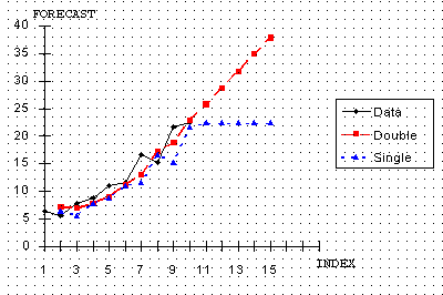
Plot comparing single and double exponential smoothing forecasts

A plot of these results (using the forecasted double smoothing values) is very enlightening.

This graph indicates that double smoothing follows the data much closer than single smoothing. Furthermore, for forecasting single smoothing cannot do better than projecting a straight horizontal line, which is not very likely to occur in reality. So in this case double smoothing is preferred.

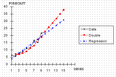
Plot comparing double exponential smoothing and regression forecasts

Finally, let us compare double smoothing with linear regression:

This is an interesting picture. Both techniques follow the data in similar fashion, but the regression line is more conservative. That is, there is a slower increase with the regression line than with double smoothing.

Selection of technique depends on the forecaster

The selection of the technique depends on the forecaster. If it is desired to portray the growth process in a more aggressive manner, then one selects double smoothing. Otherwise, regression may be preferable. It should be noted that in linear regression "time" functions as the independent variable. Chapter 4 discusses the basics of linear regression, and the details of regression estimation.