6.
Process or Product Monitoring and Control
6.4.
Introduction to Time Series Analysis
6.4.3.
What is Exponential Smoothing?
6.4.3.2.
|
Forecasting with Single Exponential Smoothing
|
|
|
|
Forecasting Formula
|
|
Forecasting the next point
|
The forecasting formula is the basic equation
$$ S_{t+1} = \alpha y_t + (1-\alpha) S_t, \,\,\,\,\, 0 < \alpha \le 1, \,\,\,\,\, t > 0 \, . $$
|
|
New forecast is previous forecast plus an error adjustment
|
This can be written as:
$$ S_{t+1} = S_t + \alpha \epsilon_t \, , $$
where \(\epsilon_t\)
is the forecast error (actual - forecast) for
period \(t\).
In other words, the new forecast is the old one plus an adjustment
for the error that occurred in the last forecast.
|
|
|
Bootstrapping of Forecasts
|
|
Bootstrapping forecasts
|
What happens if you wish to forecast from some origin, usually the
last data point, and no actual observations are available? In this
situation we have to modify the formula to become:
$$ S_{t+1} = \alpha y_{orgin} + (1-\alpha) S_t \, , $$
where \(y_{origin}\)
remains constant. This technique is known as bootstrapping.
|
|
|
Example of Bootstrapping
|
|
Example
|
The last data point in the previous example was 70 and its forecast
(smoothed value \(S\))
was 71.7. Since we do have the data point
and the forecast available, we can calculate the next forecast
using the regular formula with \(\alpha = 0.1\) as
$$ \begin{eqnarray}
S_{t+1} & = & \alpha y_{orgin} + (1-\alpha) S_t \\
& = & 0.1(70) + 0.9(71.7) \\
& = & 71.5 \, .
\end{eqnarray} $$
But for the next forecast we have no data point (observation).
So now we compute:
$$ S_{t+2} = 0.1(70) + 0.9(71.5) = 71.35 \, . $$
|
|
|
Comparison between bootstrap and regular forecasting
|
|
Table comparing two methods
|
The following table displays the comparison between the two methods:
|
Period
|
Bootstrap
forecast
|
Data
|
Single Smoothing
Forecast
|
|
|
13
|
71.50
|
75
|
71.5
|
|
14
|
71.35
|
75
|
71.9
|
|
15
|
71.21
|
74
|
72.2
|
|
16
|
71.09
|
78
|
72.4
|
|
17
|
70.98
|
86
|
73.0
|
|
|
|
Single Exponential Smoothing with Trend
|
|
|
Single Smoothing (short for single exponential smoothing) is not very
good when there is a trend. The single coefficient \(\alpha\)
is not enough.
|
|
Sample data set with trend
|
Let us demonstrate this with the following data set smoothed with an \(\alpha\)
of 0.3:
|
Data
|
Fit
|
|
|
6.4
|
|
|
5.6
|
6.4
|
|
7.8
|
6.2
|
|
8.8
|
6.7
|
|
11.0
|
7.3
|
|
11.6
|
8.4
|
|
16.7
|
9.4
|
|
15.3
|
11.6
|
|
21.6
|
12.7
|
|
22.4
|
15.4
|
|
|
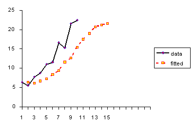
Plot demonstrating inadequacy of single exponential smoothing
when there is trend
|
The resulting graph looks like:

|


