|
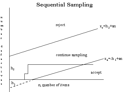
Description of sequentail sampling graph
|
The cumulative observed number of defectives is plotted on the graph.
For each point, the x-axis is the total number of items thus far
selected, and the y-axis is the total number of observed defectives.
If the plotted point falls within the parallel lines the process
continues by drawing another sample. As soon as a point falls on or
above the upper line, the lot is rejected. And when a point falls on
or below the lower line, the lot is accepted. The process can
theoretically last until the lot is 100% inspected. However, as a
rule of thumb, sequential-sampling plans are truncated after the
number inspected reaches three times the number that would have
been inspected using a corresponding single sampling plan.
|
|
Equations for the limit lines
|
The equations for the two limit lines are functions of the
parameters \(p_1\), \(\alpha\), \(p_2\), and \(\beta\).
$$ \begin{eqnarray}
x_a & = & -h_1 + s n \\
x_r & = & h_2 + s n \, ,
\end{eqnarray} $$
where
$$ \begin{eqnarray}
k & = & \mbox{log} \left[ \frac{p_2(1-p_1)}{p_1(1-p_2)}\right] \\
h_1 & = & \frac{1}{k} \left[ \mbox{log} \left(\frac{1-\alpha}{\beta}\right) \right] \\
h_2 & = & \frac{1}{k} \left[ \mbox{log} \left(\frac{1-\beta}{\alpha}\right) \right] \\
s & = & \frac{1}{k} \left[ \mbox{log} \left(\frac{1-p_1}{1-p_2}\right) \right] \, .
\end{eqnarray} $$
Instead of using the graph to determine the fate of the lot, one can
resort to generating tables (with the help of a computer program).
|
|
Example of a sequential sampling plan
|
As an example, let \(p_1 = 0.01\), \(p_2 = 0.10\), \(\alpha = 0.05\),
and \(\beta = 0.10\).
The resulting equations are:
$$ \begin{eqnarray}
x_a & = & -0.939 + 0.04 n \\
x_r & = & 1.205 + 0.04 n \, .
\end{eqnarray} $$
Both acceptance numbers and rejection numbers must be integers. The
acceptance number is the next integer less than or equal to \(x_a\)
and the rejection number is the next integer
greater than or equal to \(x_r\).
Thus for \(n=1\),
the acceptance number is -1, which is impossible, and the
rejection number is 2, which is also impossible. For \(n = 24\),
the acceptance number is 0 and the rejection number is 3.
The results for \(n = 1, \, 2, \, 3, \, \ldots, \, 26\)
are tabulated below.
\(n\)
inspect
|
\(n\)
accept
|
\(n\)
reject
|
\(n\)
inspect
|
\(n\)
accept
|
\(n\)
reject
|
|
|
1
|
x
|
x
|
14
|
x
|
2
|
|
2
|
x
|
2
|
15
|
x
|
2
|
|
3
|
x
|
2
|
16
|
x
|
2
|
|
4
|
x
|
2
|
17
|
x
|
2
|
|
5
|
x
|
2
|
18
|
x
|
2
|
|
6
|
x
|
2
|
19
|
x
|
2
|
|
7
|
x
|
2
|
20
|
x
|
3
|
|
8
|
x
|
2
|
21
|
x
|
3
|
|
9
|
x
|
2
|
22
|
x
|
3
|
|
10
|
x
|
2
|
23
|
x
|
3
|
|
11
|
x
|
2
|
24
|
0
|
3
|
|
12
|
x
|
2
|
25
|
0
|
3
|
|
13
|
x
|
2
|
26
|
0
|
3
|
So, for \(n=24\)
the acceptance number is 0 and the rejection
number is 3. The "x" means that acceptance or rejection is not
possible.
Other sequential plans are given below.
\(n\)
inspect
|
\(n\)
accept
|
\(n\)
reject
|
|
|
49
|
1
|
3
|
|
58
|
1
|
4
|
|
74
|
2
|
4
|
|
83
|
2
|
5
|
|
100
|
3
|
5
|
|
109
|
3
|
6
|
The corresponding single sampling plan is (52,2) and double sampling
plan is (21,0), (21,1).
|


