2.6.5.2.3.

Fit with deleted points

Fit with Deleted Points

Instead of the bisquare weighting, we can simply choose to delete specific points from the analysis. Based on the 4-plots above, we can delete points with an absolute value for the residual greater than 0.1. This resulted in two points being deleted from the analysis. Dataplot generated the following output for the fit.

LEAST SQUARES POLYNOMIAL FIT
SAMPLE SIZE N       =       78
DEGREE              =        2
REPLICATION CASE
REPLICATION STANDARD DEVIATION =     0.1954713464D-01
REPLICATION DEGREES OF FREEDOM =          70
NUMBER OF DISTINCT SUBSETS     =           8
  
  
        PARAMETER ESTIMATES           (APPROX. ST. DEV.)    T VALUE
 1  A0                 -0.144441       (0.1754E-01)         -8.2
 2  A1                  0.217116       (0.6757E-03)         0.32E+03
 3  A2                 -0.436235E-03   (0.5553E-05)         -79.
  
RESIDUAL    STANDARD DEVIATION =         0.0281810053
RESIDUAL    DEGREES OF FREEDOM =          75

The fitted quadratic model with the points deleted is

The residual standard deviation is 0.028.

Plot of Predicted Values with Raw Data

To assess the model, we generate the plot of the predicted values with the raw data.

4-Plot of Residuals

We again use the 4-plot to do a residual analysis.

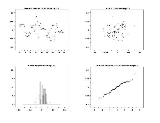
This 4-plot shows that there are no major violations of the regression assumptions.