2.6.5.2.2.

Bisquare weighting

Bisquare weighting

An alternative weighting scheme is to weight the residuals using a bisquare. We first compute the residuals from the unweighted fit and then apply the following weight function:

where m is the median absolute deviation of the residuals. The weight is set to 0 if the absolute value of the residual is greater than 6m.

This method provides an effective alternative to deleting specific points. Extreme outliers are deleted, but mild outliers are downweighted rather than deleted altogether. The analysis is shown below.

Quadratic Fit with Bisquare Weighting of the Residuals

Given the standard deviation plot and the plot of the power function, using a bisquare weighting of the residuals is a reasonable approach for this data set. Dataplot generated the following output after applying the bisquare weighting.

LEAST SQUARES POLYNOMIAL FIT
SAMPLE SIZE N       =       80
DEGREE              =        2
REPLICATION CASE
REPLICATION STANDARD DEVIATION =     0.2554919757D-01
REPLICATION DEGREES OF FREEDOM =          72
NUMBER OF DISTINCT SUBSETS     =           8
  
  
        PARAMETER ESTIMATES           (APPROX. ST. DEV.)    T VALUE
 1  A0                 -0.147403       (0.1543E-01)         -9.6
 2  A1                  0.217221       (0.6020E-03)         0.36E+03
 3  A2                 -0.436653E-03   (0.4978E-05)         -88.
  
RESIDUAL    STANDARD DEVIATION =         0.0241919290
RESIDUAL    DEGREES OF FREEDOM =          77

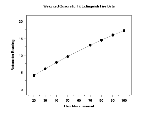
The fitted weighted quadratic model is

Plot of Predicted Values with Raw Data

To assess the model, we generate the plot of the predicted values with the raw data.

This plot indicates a good fit.

4-Plot of Residuals

We again use the 4-plot to do a residual analysis.

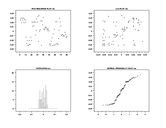
This 4-plot shows that applying the bisquare weighting scheme makes little practical difference in this case.