2. Measurement Process Characterization
2.3. Calibration
2.3.3. Calibration designs
2.3.3.2. General solutions to calibration designs

2.3.3.2.1.

General matrix solutions to calibration designs

Requirements

Solutions for all designs that are cataloged in this Handbook are included with the designs. Solutions for other designs can be computed from the instructions below given some familiarity with matrices. The matrix manipulations that are required for the calculations are:

• transposition (indicated by ')
• multiplication
• inversion

Notation

• n = number of difference measurements
• m = number of artifacts
• (n - m + 1) = degrees of freedom
• X= (nxm) design matrix
• r'= (mx1) vector identifying the restraint
• = (mx1) vector identifying ith item of interest consisting of a 1 in the ith position and zeros elsewhere
• R*= value of the reference standard
• Y= (mx1) vector of observed difference measurements

Convention for showing the measurement sequence

The convention for showing the measurement sequence is illustrated with the three measurements that make up a 1,1,1 design for 1 reference standard, 1 check standard, and 1 test item. Nominal values are underlined in the first line .

                 1     1     1
          Y(1) = +     -

          Y(2) = +           -

          Y(3) =       +     -

Matrix algebra for solving a design

The (mxn) design matrix X is constructed by replacing the pluses (+), minues (-) and blanks with the entries 1, -1, and 0 respectively.

The (mxm) matrix of normal equations, X'X, is formed and augmented by the restraint vector to form an (m+1)x(m+1) matrix, A:

Inverse of design matrix

The A matrix is inverted and shown in the form:

where Q is an mxm matrix that, when multiplied by s², yields the usual variance-covariance matrix.

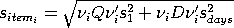
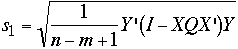
Estimates of values of individual artifacts

The least-squares estimates for the values of the individual artifacts are contained in the (mx1) matrix, B, where

where Q is the upper left element of the A^-1 matrix shown above. The structure of the individual estimates is contained in the QX' matrix; i.e. the estimate for the ith item can be computed from XQ and Y by

• Cross multiplying the ith column of XQ with Y
• And adding R*(nominal test)/(nominal restraint)

Clarify with an example

We will clarify the above discussion with an example from the mass calibration process at NIST. In this example, two NIST kilograms are compared with a customer's unknown kilogram.

The design matrix, X, is

The first two columns represent the two NIST kilograms while the third column represents the customers kilogram (i.e., the kilogram being calibrated).

The measurements obtained, i.e., the Y matrix, are

The measurements are the differences between two measurements, as specified by the design matrix, measured in grams. That is, Y(1) is the difference in measurement between NIST kilogram one and NIST kilogram two, Y(2) is the difference in measurement between NIST kilogram one and the customer kilogram, and Y(3) is the difference in measurement between NIST kilogram two and the customer kilogram.

The value of the reference standard, R^*, is 0.82329.

Then

If there are three weights with known values for weights one and two, then

r = [ 1    1    0 ]

Thus

and so

From A^-1, we have

We then compute QX'

We then compute B = QX'Y + h'R^*

This yields the following least-squares coefficient estimates:

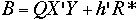
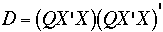
Standard deviations of estimates

The standard deviation for the ith item is:

where

The process standard deviation, which is a measure of the overall precision of the (NIST) mass calibrarion process,

is the residual standard deviation from the design, and s_days is the standard deviation for days, which can only be estimated from check standard measurements.

Example

We continue the example started above. Since n = 3 and m = 3, the formula reduces to:

Substituting the values shown above for X, Y, and Q results in

and

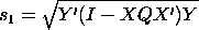
Y'(I - XQX')Y = 0.0000083333

Finally, taking the square root gives

s₁ = 0.002887

The next step is to compute the standard deviation of item 3 (the customers kilogram), that is s_item3. We start by substitituting the values for X and Q and computing D

Next, we substitute = [0 0 1] and = 0.02111² (this value is taken from a check standard and not computed from the values given in this example).

We obtain the following computations

and

and