1. Exploratory Data Analysis
1.4. EDA Case Studies
1.4.2. Case Studies
1.4.2.7. Standard Resistor

1.4.2.7.3.

Quantitative Output and Interpretation

Summary Statistics

As a first step in the analysis, common summary statistics are computed from the data.

      Sample size  = 1000
      Mean         =   28.01634  
      Median       =   28.02910
      Minimum      =   27.82800
      Maximum      =   28.11850    
      Range        =    0.29050
      Stan. Dev.   =    0.06349

Location

One way to quantify a change in location over time is to fit a straight line to the data using an index variable as the independent variable in the regression. For our data, we assume that data are in sequential run order and that the data were collected at equally spaced time intervals. In our regression, we use the index variable X = 1, 2, ..., N, where N is the number of observations. If there is no significant drift in the location over time, the slope parameter should be zero.

      Coefficient     Estimate     Stan. Error      t-Value
          B0           27.9114      0.1209E-02     0.2309E+05
          B1        0.20967E-03     0.2092E-05        100.2
 
      Residual Standard Deviation = 0.1909796E-01
      Residual Degrees of Freedom = 998

The slope parameter, B₁, has a t value of 100.2 which is statistically significant. The value of the slope parameter estimate is 0.00021. Although this number is nearly zero, we need to take into account that the original scale of the data is from about 27.8 to 28.2. In this case, we conclude that there is a drift in location.

Variation

One simple way to detect a change in variation is with a Bartlett test after dividing the data set into several equal-sized intervals. However, the Bartlett test is not robust for non-normality. Since the normality assumption is questionable for these data, we use the alternative Levene test. In particular, we use the Levene test based on the median rather the mean. The choice of the number of intervals is somewhat arbitrary, although values of four or eight are reasonable. We will divide our data into four intervals.

      H0:  σ12 = σ22 = σ32 = σ42  
      Ha:  At least one σi2 is not equal to the others.

      Test statistic:  W = 140.85
      Degrees of freedom:  k - 1 = 3
      Significance level:  α = 0.05
      Critical value:  Fα,k-1,N-k = 2.614
      Critical region:  Reject H0 if W > 2.614

In this case, since the Levene test statistic value of 140.85 is greater than the 5 % significance level critical value of 2.614, we conclude that there is significant evidence of nonconstant variation.

Randomness

There are many ways in which data can be non-random. However, most common forms of non-randomness can be detected with a few simple tests. The lag plot in the 4-plot in the previous section is a simple graphical technique.

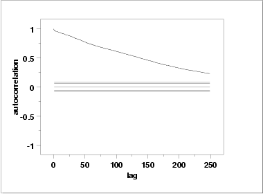
One check is an autocorrelation plot that shows the autocorrelations for various lags. Confidence bands can be plotted at the 95 % and 99 % confidence levels. Points outside this band indicate statistically significant values (lag 0 is always 1).

The lag 1 autocorrelation, which is generally the one of greatest interest, is 0.97. The critical values at the 5 % significance level are -0.062 and 0.062. This indicates that the lag 1 autocorrelation is statistically significant, so there is strong evidence of non-randomness.

A common test for randomness is the runs test.

      H0:  the sequence was produced in a random manner
      Ha:  the sequence was not produced in a random manner  

      Test statistic:  Z = -30.5629
      Significance level:  α = 0.05
      Critical value:  Z1-α/2 = 1.96 
      Critical region:  Reject H0 if |Z| > 1.96   

Because the test statistic is outside of the critical region, we reject the null hypothesis and conclude that the data are not random.

Distributional Analysis

Since we rejected the randomness assumption, the distributional tests are not meaningful. Therefore, these quantitative tests are omitted. Since the Grubbs' test for outliers also assumes the approximate normality of the data, we omit Grubbs' test as well.

Univariate Report

It is sometimes useful and convenient to summarize the above results in a report.

 Analysis for resistor case study
  
 1: Sample Size                           = 1000
  
 2: Location
    Mean                                  = 28.01635
    Standard Deviation of Mean            = 0.002008
    95% Confidence Interval for Mean      = (28.0124,28.02029)
    Drift with respect to location?       = NO
  
 3: Variation
    Standard Deviation                    = 0.063495
    95% Confidence Interval for SD        = (0.060829,0.066407)
    Change in variation?
    (based on Levene's test on quarters
    of the data)                          = YES
  
 4: Randomness
    Autocorrelation                       = 0.972158
    Data Are Random?
      (as measured by autocorrelation)    = NO
  
 5: Distribution
    Distributional test omitted due to
    non-randomness of the data
  
 6: Statistical Control
    (i.e., no drift in location or scale,
    data are random, distribution is 
    fixed)
    Data Set is in Statistical Control?   = NO
  
 7: Outliers?
    (Grubbs' test omitted due to
    non-randomness of the data)