1. Exploratory Data Analysis
1.4. EDA Case Studies
1.4.2. Case Studies
1.4.2.5. Beam Deflections

1.4.2.5.3.

Develop a Better Model

Sinusoidal Model

The lag plot and autocorrelation plot in the previous section strongly suggested a sinusoidal model might be appropriate. The basic sinusoidal model is:

where C is constant defining a mean level, is an amplitude for the sine function, is the frequency, T_i is a time variable, and is the phase. This sinusoidal model can be fit using non-linear least squares.

To obtain a good fit, sinusoidal models require good starting values for C, the amplitude, and the frequency.

Good Starting Value for C

A good starting value for C can be obtained by calculating the mean of the data. If the data show a trend, i.e., the assumption of constant location is violated, we can replace C with a linear or quadratic least squares fit. That is, the model becomes

or

Since our data did not have any meaningful change of location, we can fit the simpler model with C equal to the mean. From the summary output in the previous page, the mean is -177.44.

Good Starting Value for Frequency

The starting value for the frequency can be obtained from the spectral plot, which shows the dominant frequency is about 0.3.

Complex Demodulation Phase Plot

The complex demodulation phase plot can be used to refine this initial estimate for the frequency.

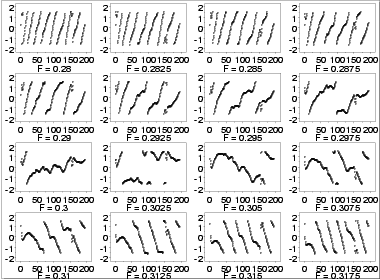
For the complex demodulation plot, if the lines slope from left to right, the frequency should be increased. If the lines slope from right to left, it should be decreased. A relatively flat (i.e., horizontal) slope indicates a good frequency. We could generate the demodulation phase plot for 0.3 and then use trial and error to obtain a better estimate for the frequency. To simplify this, we generate 16 of these plots on a single page starting with a frequency of 0.28, increasing in increments of 0.0025, and stopping at 0.3175.

Interpretation

The plots start with lines sloping from left to right but gradually change to a right to left slope. The relatively flat slope occurs for frequency 0.3025 (third row, second column). The complex demodulation phase plot restricts the range from to . This is why the plot appears to show some breaks.

Good Starting Values for Amplitude

The complex demodulation amplitude plot is used to find a good starting value for the amplitude. In addition, this plot indicates whether or not the amplitude is constant over the entire range of the data or if it varies. If the plot is essentially flat, i.e., zero slope, then it is reasonable to assume a constant amplitude in the non-linear model. However, if the slope varies over the range of the plot, we may need to adjust the model to be:

That is, we replace with a function of time. A linear fit is specified in the model above, but this can be replaced with a more elaborate function if needed.

Complex Demodulation Amplitude Plot

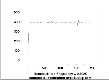
The complex demodulation amplitude plot for this data shows that:

1. The amplitude is fixed at approximately 390.
2. There is a short start-up effect.
3. There is a change in amplitude at around x=160 that should be investigated for an outlier.

In terms of a non-linear model, the plot indicates that fitting a single constant for should be adequate for this data set.

Fit Output

Using starting estimates of 0.3025 for the frequency, 390 for the amplitude, and -177.44 for C, Dataplot generated the following output for the fit.

 LEAST SQUARES NON-LINEAR FIT
       SAMPLE SIZE N =      200
       MODEL--Y =C + AMP*SIN(2*3.14159*FREQ*T + PHASE)
       NO REPLICATION CASE
  
 ITERATION  CONVERGENCE  RESIDUAL  *  PARAMETER
  NUMBER      MEASURE    STANDARD  *  ESTIMATES
                         DEVIATION *
 ----------------------------------*-----------
     1--  0.10000E-01  0.52903E+03 *-0.17743E+03 0.39000E+03 0.30250E+00 0.10000E+01
     2--  0.50000E-02  0.22218E+03 *-0.17876E+03-0.33137E+03 0.30238E+00 0.71471E+00
     3--  0.25000E-02  0.15634E+03 *-0.17886E+03-0.24523E+03 0.30233E+00 0.14022E+01
     4--  0.96108E-01  0.15585E+03 *-0.17879E+03-0.36177E+03 0.30260E+00 0.14654E+01
  
         FINAL PARAMETER ESTIMATES           (APPROX. ST. DEV.)    T VALUE
        1  C                   -178.786       ( 11.02    )       -16.22
        2  AMP                 -361.766       ( 26.19    )       -13.81
        3  FREQ                0.302596       (0.1510E-03)        2005.
        4  PHASE                1.46536       (0.4909E-01)        29.85
  
       RESIDUAL    STANDARD DEVIATION =         155.8484
       RESIDUAL    DEGREES OF FREEDOM =         196

Model

From the fit output, our proposed model is: We will evaluate the adequacy of this model in the next section.