8.4.2.1. Graphical estimation

8. Assessing Product Reliability
8.4. Reliability Data Analysis
8.4.2. How do you fit an acceleration model?

8.4.2.1. Graphical estimation

This section will discuss the following:

How to fit an Arrhenius model with graphical estimation
Graphical estimation: an Arrhenius model example
Fitting more complicated models

Estimate acceleration model parameters by estimating cell $T_{50}$ values (or $\alpha$ values) and then using regression to fit the model across the cells

How to fit an Arrhenius Model with Graphical Estimation

Graphical methods work best (and are easiest to describe) for a simple one-stress model like the widely used Arrhenius model $$ t_f = A \cdot \mbox{ exp } \left( \frac{\Delta H}{kT} \right) \, , $$ with $T$ denoting temperature measured in degrees Kelvin (273.16 + degrees Celsius) and $k$ is Boltzmann's constant (8.617 × 10^-5 in eV/K).

When applying an acceleration model to a distribution of failure times, we interpret the deterministic model equation to apply at any distribution percentile we want. This is equivalent to setting the life distribution scale parameter equal to the model equation ($T_{50}$ for the lognormal, $\alpha$ for the Weibull and the MTBF, or $1/\lambda$ for the exponential). For the lognormal, for example, we have $$ T_{50} = A \cdot \mbox{ exp } \left( \frac{\Delta H}{kT} \right) \, , $$ $$ \mbox{ln } T_{50} = y = \mbox{ln } A + \Delta H \left( \frac{1}{kT} \right) \, . $$ This can be written as $$ y = a + bx $$ with $$ b = \Delta H \,\,\,\,\, \mbox{ and } \,\,\,\,\, x = \frac{1}{kT} \, . $$ So, if we run several stress cells and compute $T_{50}$ values for each cell, a plot of the natural log of these $T_{50}$ values versus the corresponding $1/kT$ values should be roughly linear with a slope of $\Delta H$ and an intercept of $\mbox{ln } A$. In practice, a computer fit of a line through these points is typically used to obtain the Arrhenius model estimates. Remember that $T$ is in Kelvin in the above equations. For temperature in Celsius, use the following for $1/kT$: 11605/($t$°C + 273.16).

An example will illustrate the procedure.

Graphical Estimation: An Arrhenius Model Example:

Arrhenius model example

Component life tests were run at three temperatures: 85 °C, 105 °C and
125 °C. The lowest temperature cell was populated with 100 components; the 105 °C cell had 50 components and the highest stress cell had 25 components. All tests were run until either all the units in the cell had failed or 1000 hours was reached. Acceleration was assumed to follow an Arrhenius model and the life distribution model for the failure mode was believed to be lognormal. The normal operating temperature for the components is 25 °C and it is desired to project the use CDF at 100,000 hours.

Test results:

Cell 1 (85 °C): 5 failures at 401, 428, 695, 725 and 738 hours. Ninety-five units were censored at 1000 hours running time.

Cell 2 (105 °C): 35 failures at 171, 187, 189, 266, 275, 285, 301, 302, 305, 316, 317, 324, 349, 350, 386, 405, 480, 493, 530, 534, 536, 567, 589, 598, 599, 614, 620, 650, 668, 685, 718, 795, 854, 917, and 926 hours. Fifteen units were censored at 1000 hours running time.

Cell 3 (125 °C): 24 failures at 24, 42, 92, 93, 141, 142, 143, 159, 181, 188, 194, 199, 207, 213, 243, 256, 259, 290, 294, 305, 392, 454, 502 and 696. One unit was censored at 1000 hours running time.

Failure analysis confirmed that all failures were due to the same failure mechanism (if any failures due to another mechanism had occurred, they would have been considered censored run times in the Arrhenius analysis).

Steps to Fitting the Distribution Model and the Arrhenius Model:

Do plots for each cell and estimate $T_{50}$ and sigma as previously discussed.
Plot all the cells on the same graph and check whether the lines are roughly parallel (a necessary consequence of true acceleration).
If probability plots indicate that the lognormal model is appropriate and that sigma is consistant among cells, plot $\mbox{ln } T_{50}$ versus
11605/($t$ °C + 273.16) for each cell, check for linearity and fit a straight line through the points. Since the points have different values of precision, due to different numbers of failures in each cell, it is recommended that the number of failures in each cell be used as weights in a regression when fitting a line through the points.
Use the slope of the line as the $\Delta H$ estimate and calculate the Arrhenius A constant from the intercept using $A = e^{intercept}$.
Estimate the common sigma across all the cells by the weighted average of the individual cell sigma estimates. Use the number of failures in a cell divided by the total number of failures in all cells as that cell's weight. This will allow cells with more failures to play a bigger role in the estimation process.

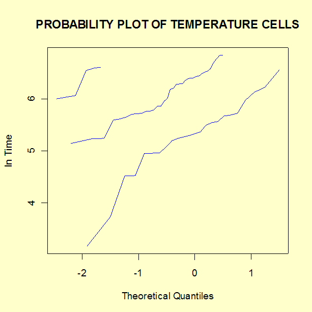
Solution for Arrhenius model example

Analysis of Multicell Arrhenius Model Data:

The following lognormal probability plot was generated for our data so that all three stress cells are plotted on the same graph.

Lognormal probability plots of temperature cells

Note that the lines are somewhat straight (a check on the lognormal model) and the slopes are approximately parallel (a check on the acceleration assumption).

The cell $\mbox{ln } T_{50}$ and sigma estimates are obtained from linear regression fits for each cell using the data from the probability plot. Each fit will yield a cell $A_0$, the $\mbox{ln } T_{50}$ estimate, and $A_1$, the cell sigma estimate. These are summarized in the table below.

**Summary of Least Squares Estimation of Cell Lognormal Parameters**
Cell Number	$\mbox{ln } T_{50}$	Sigma
1 ($t$ °C = 85)	8.168	0.908
2 ($t$ °C = 105)	6.415	0.663
3 ($t$ °C = 125)	5.319	0.805

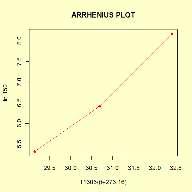
The three cells have 11605/($t$ °C + 273.16) values of 32.40, 30.69 and 29.15 respectively, in cell number order. The Arrhenius plot is

With only three cells, it is unlikely a straight line through the points will present obvious visual lack of fit. However, in this case, the points appear to line up very well.

Finally, the model coefficients are computed from a weighted linear fit of $\mbox{ln } T_{50}$ versus 11605/($t$ °C + 273.16), using weights of 5, 35, and 24 for each cell. This will yield a $\mbox{ln } A$ estimate of -18.312 ($A = e^{-18.312} = 0.1115 \times 10^{-7}$) and a $\Delta H$ estimate of 0.808. With this value of $\Delta H $, the acceleration between the lowest stress cell of 85 °C and the highest of 125 °C is $$ \mbox{exp } \left[ 0.808 \times 11605 \times \left( \frac{1}{358.16} - \frac{1}{398.16} \right) \right] = 13.9 \, , $$ which is almost 14 × acceleration. Acceleration from 125 °C to the use condition of 25 °C is 3708×. The use $T_{50}$ is $$ e^{-18.312} \times e^{0.808 \times 11605 \times 1/298.16} = e^{13.137} = 507383 \, . $$

A single sigma estimate for all stress conditions can be calculated as a weighted average of the three sigma estimates obtained from the experimental cells. The weighted average is (5/64) × 0.908 + (35/64) × 0.663 + (24/64) × 0.805 = 0.74.

The analyses in this section can can be implemented using both Dataplot code and R code.

Fitting More Complicated models

Models involving several stresses can be fit using multiple regression

Two stress models, such as the temperature/voltage model given by $$ t_f = A \cdot V^{\beta} \cdot \mbox{ exp } \left( \frac{\Delta H}{kT} \right) \, , $$ need at least four or five carefully chosen stress cells to estimate all the parameters. The Backwards L design previously described is an example of a design for this model. The bottom row of the "backward L" could be used for a plot testing the Arrhenius temperature dependence, similar to the above Arrhenius example. The right hand column could be plotted using $y = \mbox{ln } T_{50}$ and $x = \mbox{ln } V$, to check the voltage term in the model. The overall model estimates should be obtained from fitting the multiple regression model $$ Y = b_0 + b_1 X_1 + b_2 X_2 \, , $$ with $$ \begin{array}{rl} Y = \mbox{ln } T_{50}, & b_0 = \mbox{ln } A \\ & \\ b_1 = \Delta H, & X_1 = 1/kT \\ & \\ b_2 = \beta, & X_2 = \mbox{ln } V \, . \end{array} $$ Fitting this model, after setting up the data vectors, provides estimates for $b_0, \, b_1$, and $b_2$.

Three stress models, and even Eyring models with interaction terms, can be fit by a direct extension of these methods. Graphical plots to test the model, however, are less likely to be meaningful as the model becomes more complex.