8.1.9.1. NHPP power law

8. Assessing Product Reliability
8.1. Introduction
8.1.9. How can you model reliability growth?

8.1.9.1. NHPP power law

If the Power Law applies, Repair Rates improve over time according to the formula $\alpha t^{-\beta}$ The exponent $\beta$ lies between 0 and 1 and is called the reliability growth slope

This repairable system model was described in Section 8.1.7.2. The expected number of failures by time $t$ has the form $M(t) = a t^b$ and the repair rate has the form $m(t) = a b t^{b-1}$. This will model improvement when 0 $ < b < $ 1, with larger improvements coming when $b$ is smaller. As we will see in the next section on Duane Plotting, it is convenient to define $\beta = 1 - b$ and $\alpha = ab$ , and write the repair rate as $$ m(t) = \alpha t ^{-\beta} \,\, . $$ Again we have improvement when 0 $< \beta <$ 1, with larger improvement coming from larger values of $\beta$. $\beta$ is known as the Duane Plot slope or the reliability improvement Growth Slope.

In terms of the original parameters for $M(t)$, we have $$ a = \frac{\alpha}{1-\beta}\,\,\, \mbox{ and } \,\,\, b = 1-\beta \,\, . $$ Use of the Power Law model for reliability growth test data generally assumes the following:

1. While the test is ongoing, system improvements are introduced that produce continual improvements in the rate of system repair.

2. Over a long enough period of time the effect of these improvements can be modeled adequately by the continuous polynomial repair rate improvement model $\alpha t^{-\beta}$.

When an improvement test ends, the MTBF stays constant at its last achieved value

3. When the improvement test ends at test time $T$ and no further improvement actions are ongoing, the repair rate has been reduced to $\alpha T^{-\beta}$. The repair rate remains constant from then on at this new (improved) level.

Assumption three means that when the test ends, the HPP constant repair rate model takes over and the MTBF for the system from then on is the reciprocal of the final repair rate or $(T^{\beta})/\alpha$. If we estimate the expected number of failures up to time T by the actual number observed, the estimated MTBF at the end of a reliability test (following the Power Law) is: $$ \mbox{ESTIMATED MTBF AT END OF TEST } = \frac{T}{r(1-\beta)} \,\, , $$ with $T$ denoting the test time,$r$ is the total number of test failures and $\beta$ is the reliability growth slope. A formula for estimating $\beta$ from system failure times is given in the Analysis Section for the Power Law model.

Simulated Data Example

Simulating NHPP Power Law Data

Step 1: User inputs the positive constants $a$ and $b$.

Step 2: Simulate a vector of $n$ uniform (0,1) random numbers. Call these $U_1, \, U_2, \, U_3, \, \ldots, \, U_n$.

Step 3: Calculate $Y_1 = \left\{ -\frac{1}{a} \mbox{ ln } U_1 \right\}^{1/b}$.

Step $i$: Calculate $Y_i = \left\{ Y_{i-1}^b - \frac{1}{a} \mbox{ ln } U_i \right\}^{1/b} $ for $i$ = 2, ..., $n$.

The $n$ numbers $Y_1, \, Y_2, \, \ldots, \, Y_n$ are the desired repair times simulated from an NHPP Power Law process with parameters $a, \, b$ (or $\beta = 1-b$ and $\alpha = ab$).

Example

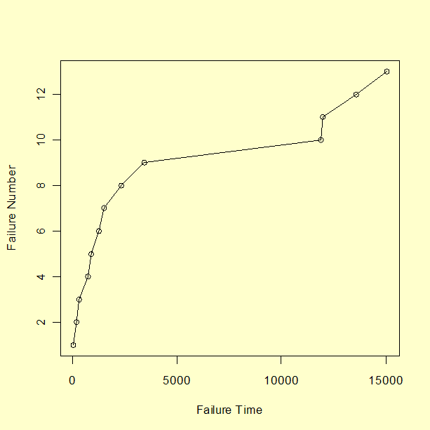
We generated $n$ = 13 random repair times using the NHPP Power Law process with $a$ = 0.2 and $b$ = 0.4. The resulting data and a plot of failure number versus repair times are shown below.

Failure	Failure
Number	Time
1	26
2	182
3	321
4	728
5	896
6	1268
7	1507
8	2325
9	3427
10	11871
11	11978
12	13562
13	15053

The NHPP power law process can be implemented using both Dataplot code and R code.