IGPDF

IGPDF (LET)

Library Function

Compute the inverse Gaussian probability density function with shape parameters and .

The inverse Gaussian distribution has the following probability density function:

with and denoting the shape parameters.

The inverse Gaussian distribution has mean and standard deviation .

The inverse Gaussian distribution can be generalized with location and scale parameters in the usual way.

LET <y> = IGPDF(<x>,<gamma>,<mu>,<loc>,<scale>)
                        <SUBSET/EXCEPT/FOR qualification>
where <x> is a variable or a parameter;
            <gamma> is number or parameter that specifies the first shape parameter;
            <mu> is number or parameter that specifies the second shape parameter;
            <loc> is number or parameter that specifies the location parameter;
            <scale> is number or parameter that specifies the scale parameter;
            <y> is a variable or a parameter (depending on what <x> is) where the computed inverse Gaussian pdf value is stored;
and where the <SUBSET/EXCEPT/FOR qualification> is optional.

Note that the location and scale parameters are optional.

LET A = IGPDF(3,2,1)
LET A = IGPDF(A1,2,1)
LET X2 = IGPDF(X1,2,3)
PLOT IGPDF(X,2,1.5) FOR X = 0.1 0.1 5

Random numbers, probability plots, and Kolmogorov-Smirnov and chi-square goodness of fit tests can be generated with the commands:
LET GAMMA = <value>
LET MU = <value>
LET Y = INVERSE GAUSSIAN RANDOM NUMBERS FOR I = 1 1 N
INVERSE GAUSSIAN PROBABILITY PLOT Y
INVERSE GAUSSIAN KOLMOGOROV-SMIRNOV GOODNESS OF FIT Y
INVERSE GAUSSIAN CHI-SQUARE FIT Y


The following commands can be used to generate estimates for the shape parameters of the inverse Gaussian distribution:

LET GAMMA1 = <value>
LET GAMMA2 = <valuee>
LET MU1 = <value>
LET MU2 = <value>
INVERSE GAUSSIAN PPCC PLOT Y
INVERSE GAUSSIAN KS PLOT Y


The default values for GAMMA1 and GAMMA2 are 0.5 and 25. The default values for MU1 and MU2 are 0.5 and 25.

Maximum likelihood estimates can be obtained by entering the command

INVERSE GAUSSIAN MAXIMUM LIKELIHOOD Y

The maximum likelihood estimates are





with and n denoting the sample mean and sample size, respectively.

The inverse Gaussian distribution is symmetric and moderate tailed for small . It is highly skewed and long tailed for large . It approaches normality as gamma approaches zero.

The case where = 1 is referred to as the Wald distribution. Enter HELP WALPDF for details.

None

None

IGCDF	= Compute the inverse Gaussian cumulative distribution function.
IGPPF	= Compute the inverse Gaussian percent point function.
CHSPDF	= Compute the chi-square probability density function.
FPDF	= Compute the F probability density function.
NORPDF	= Compute the normal probability density function.
TPDF	= Compute the t probability density function.
WEIPDF	= Compute the Weibull probability density function.
WALPDF	= Compute the Wald probability density function.
FLPDF	= Compute the fatigue life probability density function.
RIGPDF	= Compute the reciprocal inverse Gaussian probability density function.

"Continuous Univariate Distributions--Volume 1", Second Edition, Johnson, Kotz, and Balakrishnan, Wiley, 1994, chapter 15.

"Statistical Distributions", Third Edition, Evans, Hastings, and Peacock, Wiley, 2000, pp. 114-116.

Distributional Modeling

1990/5: Original implementation
2003/12: Modified to treat mu as a shape parameter instead of a location parameter

 
Y1LABEL Probability
X1LABEL X
LABEL CASE ASIS
X1LABEL DISPLACEMENT 12
Y1LABEL DISPLACEMENT 12
MULTIPLOT SCALE FACTOR 2
MULTIPLOT 2 2
MULTIPLOT CORNER COORDINATES 0 0 100 100
YLIMITS 0 1.5
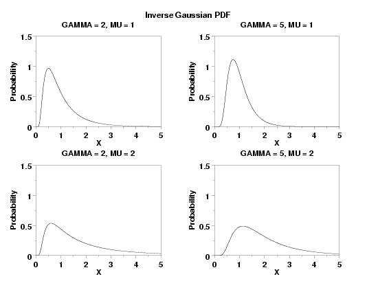
TITLE GAMMA = 2, MU = 1
PLOT IGPDF(X,2,1) FOR X = 0.01  0.01  5
TITLE GAMMA = 5, MU = 1
PLOT IGPDF(X,5,1) FOR X = 0.01  0.01  5
TITLE GAMMA = 2, MU = 2
PLOT IGPDF(X,2,2) FOR X = 0.01  0.01  5
TITLE GAMMA = 5, MU = 2
PLOT IGPDF(X,5,2) FOR X = 0.01  0.01  5
END OF MULTIPLOT
JUSTIFICATION CENTER
MOVE 50 97
CASE ASIS
TEXT Inverse Gaussian PDF