DATAPLOT Command Mode


DATAPLOT Command Mode
Dataplot Design Goals	The Dataplot language was designed with the goals of providing scientists and engineers with graphics; fitting (especially non-linear); operations with functions.
Three Core Dataplot Commands	The Dataplot command language was developed to provide a high-level, English-syntax, and self-descriptive language to perform these functions. The three core Dataplot commands are PLOT (for graphics); FIT (for linear and non-linear fitting); LET (for function operations).
Advantages of a Command Line Interface	Graphical user interfaces are increasingly becoming the preferred type of user interface for many users. Dataplot provides an alpha version of a graphical user interface (GUI) on some platforms. Graphical interfaces are helpful to new and casual users. However, a command language still provides some important advantages. Specifically, It provides portability to a large number of platforms. If a platform provides a reasonably good Fortran 77 compiler and sufficient memory, it should be possible to install Dataplot on that platform with a minimal amount of source code changes. Command languages are useful for automating routine or commonly performed tasks. Commands can be stored in ASCII files, which can be easily modfied with a standard text editor, for later use. Dataplot command files tend to be self-documenting due to the self-descriptive nature of Dataplot commands. Once you become familiar with a command language, it is typically faster to use than a mouse based interface.
Dataplot Commands Available from GUI	The choice between using the GUI interface or the command line interface is often a matter of taste. One important feature of the Dataplot graphical interface is that you can still enter any Dataplot command by simply starting to type it from the keyboard.
Example of Dataplot Command Interface Step 1: Set the Graphics Devices and Read the Data	As an example of using the command language to set your graphics device to an X11 terminal, read in a set of data, perform some basic plots and fits, and then print a Postscript version of the plots, you could enter something like the following >dataplot ECHO ON DEVICE 1 X11 DEVICE 2 POSTSCRIPT SKIP 25 READ BERGER1.DAT Y X These commands generate the following output.
Dataplot Output	THE ECHO SWITCH HAS JUST BEEN SET TO ON ************************ DEVICE 1 X11 ********************** DEVICE -- 1 I/O UNIT -- 6 MANUFACTURER --X11 MODEL -- POWER --ON CONTINUITY --ON COLOR --ON HORIZONTAL PIXELS-- 550 VERTICAL PIXELS-- 425 ***************************** DEVICE 2 POSTSCRIPT ***************************** DEVICE -- 2 I/O UNIT -- 43 MANUFACTURER --POST MODEL -- POWER --ON CONTINUITY --ON COLOR --OFF HORIZONTAL PIXELS-- 3130 VERTICAL PIXELS-- 2380 FILE NAME (LOCAL)--dppl1f.dat ***************** SKIP 25 ***************** THE NUMBER OF HEADER LINES TO BE SKIPPED HAS JUST BEEN SET TO 25 ****************************** READ BERGER1.DAT Y X ******************************** THE NUMBER OF HEADER LINES BEING SKIPPED = 25 INPUT DATA FILE SUMMARY INFORMATION-- INPUT UNIT DEVICE NUMBER = 31 INPUT FILE COLUMN LIMITS = 1 132 INPUT FILE ROW LIMITS = 1 INFINITY NUMBER OF HEADER LINES SKIPPED = 25 NUMBER OF DATA LINES READ = 107 NUMBER OF VARIABLES READ = 2 THE SCANNED REGION OF THE FIRST DATA LINE READ = 18 20.2 1 THE SCANNED REGION OF THE LAST DATA LINE READ = 45 49.0 6 VARIABLE COLUMN OBS/VARIABLE Y 1 107 X 2 107
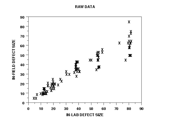
Example of Dataplot Command Interface Step 2: Plot the Data	And now enter the commands TITLE RAW DATA Y1LABEL IN-FIELD DEFECT SIZE X1LABEL IN-LAB DEFECT SIZE CHARACYER X LINE BLANK PLOT Y X
Dataplot Output	These commands generate the following output. ************************** TITLE RAW DATA ************************ THE TITLE HAS JUST BEEN SET TO RAW DATA ************************************** Y1LABEL IN-FIELD DEFECT SIZE ************************************** THE LEFT VERTICAL AXIS LABEL HAS JUST BEEN SET TO IN-FIELD DEFECT SIZE ************************************ X1LABEL IN-LAB DEFECT SIZE ************************************ THE FIRST HORIZONTAL AXIS LABEL HAS JUST BEEN SET TO IN-LAB DEFECT SIZE ********************* CHARACYER X ********************* CHARACTER 1 HAS JUST BEEN SET TO X ******************** LINE BLANK ******************** LINE 1 HAS JUST BEEN SET TO BLAN ****************** PLOT Y X ********************
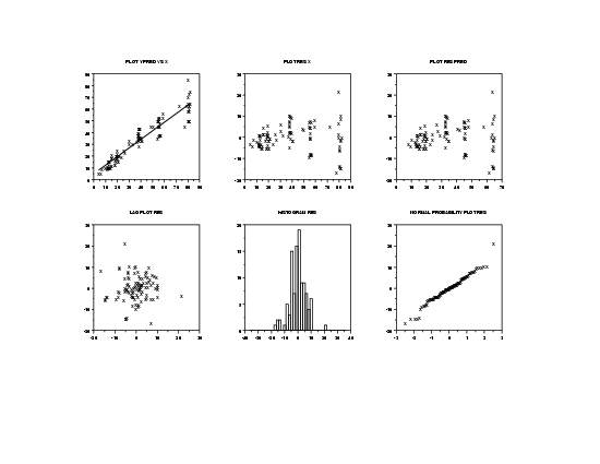
Example of Dataplot Command Interface Step 3: Fit the Data and Generate Residuals Plot	And now enter the commands LINEAR FIT Y X TITLE FITTED VALUES PLOT Y PRED VS X TITLE AUTOMATIC X1LABEL Y1LABEL 6-PLOT Y X QUIT >lpr -P<printer-id> dppl1f.dat
Dataplot Output	These commands generate the following output. ************************** LINEAR FIT Y X ************************ LEAST SQUARES POLYNOMIAL FIT SAMPLE SIZE N = 107 DEGREE = 1 REPLICATION CASE REPLICATION STANDARD DEVIATION = 0.6112687111D+01 REPLICATION DEGREES OF FREEDOM = 29 NUMBER OF DISTINCT SUBSETS = 78 PARAMETER ESTIMATES (APPROX. ST. DEV.) T VALUE 1 A0 4.99368 ( 1.126 ) 4.4 2 A1 0.731111 (0.2455E-01) 30. RESIDUAL STANDARD DEVIATION = 6.0809240341 RESIDUAL DEGREES OF FREEDOM = 105 REPLICATION STANDARD DEVIATION = 6.1126871109 REPLICATION DEGREES OF FREEDOM = 29 LACK OF FIT F RATIO = 0.9857 = THE 46.3056% POINT OF THE F DISTRIBUTION WITH 76 AND 29 DEGREES OF FREEDOM COEF AND SD(COEF) WRITTEN OUT TO FILE DPST1F.DAT SD(PRED),95LOWER,95UPPER,99LOWER,99UPPER WRITTEN OUT TO FILE DPST2F.DAT REGRESSION DIAGNOSTICS WRITTEN OUT TO FILE DPST3F.DAT PARAMETER VARIANCE-COVARIANCE MATRIX AND INVERSE OF X-TRANSPOSE X MATRIX WRITTEN OUT TO FILE DPST4F.DAT ***************************** TITLE FITTED VALUES ***************************** THE TITLE HAS JUST BEEN SET TO FITTED VALUES ************************** PLOT Y PRED VS X ************************** ************************* TITLE AUTOMATIC ************************* THE TITLE HAS JUST BEEN SET TO AUTOMATIC ***************** X1LABEL ***************** THE FIRST HORIZONTAL AXIS LABEL HAS JUST BEEN SET TO ***************** Y1LABEL ***************** THE LEFT VERTICAL AXIS LABEL HAS JUST BEEN SET TO ******************** 6-PLOT Y X **********************
Privacy Policy/Security Notice Disclaimer \| FOIA NIST is an agency of the U.S. Commerce Department. Date created: 06/05/2001 Last updated: 09/20/2016 Please email comments on this WWW page to alan.heckert@nist.gov.