5. Process Improvement
5.1. Introduction

5.1.1.

What is experimental design?

Experimental Design (or DOE) economically maximizes information

In an experiment, we deliberately change one or more process variables (or factors) in order to observe the effect the changes have on one or more response variables. The (statistical) design of experiments (DOE) is an efficient procedure for planning experiments so that the data obtained can be analyzed to yield valid and objective conclusions. 

DOE begins with determining the objectives of an experiment and selecting the process factors for the study. An Experimental Design is the laying out of a detailed experimental plan in advance of doing the experiment. Well chosen experimental designs maximize the amount of "information" that can be obtained for a given amount of experimental effort. 

The statistical theory underlying DOE generally begins with the concept of process models.

Process Models for DOE

Black box process model

It is common to begin with a process model of the `black box' type, with several discrete or continuous input factors that can be controlled--that is, varied at will by the experimenter--and one or more measured output responses. The output responses are assumed continuous. Experimental data are used to derive an empirical (approximation) model linking the outputs and inputs. These empirical models generally contain first and second-order terms.

Often the experiment has to account for a number of uncontrolled factors that may be discrete, such as different machines or operators, and/or continuous such as ambient temperature or humidity. Figure 1.1 illustrates this situation.

Schematic for a typical process with controlled inputs, outputs, discrete uncontrolled factors and continuous uncontrolled factors

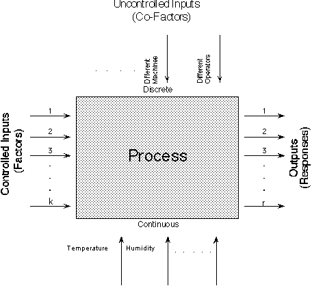
FIGURE 1.1  A `Black Box' Process Model Schematic

Models for DOE's

The most common empirical models fit to the experimental data take either a linear form or quadratic form.

Linear model

A linear model with two factors, X₁ and X₂, can be written as

\( Y = \beta_{0} + \beta_{1}X_{1} + \beta_{2}X_{2} + \beta_{12}X_{1}X_{2} + \mbox{experimental error} \)

Here, Y is the response for given levels of the main effects X₁ and X₂ and the X₁X₂ term is included to account for a possible interaction effect between X₁ and X₂. The constant \( \beta_{0} \) is the response of Y when both main effects are 0.

For a more complicated example, a linear model with three factors X₁, X₂, X₃ and one response, Y, would look like (if all possible terms were included in the model)

\( Y = \beta_{0} + \beta_{1}X_{1} + \beta_{2}X_{2} + \beta_{3}X_{3} + \beta_{12}X_{1}X_{2} + \\ \beta_{13}X_{1}X_{3} + \beta_{23}X_{2}X_{3} + \beta_{123}X_{1}X_{2}X_{3} + \\ \mbox{experimental error} \)

The three terms with single "X's" are the main effects terms. There are k(k-1)/2 = 3*2/2 = 3 two-way interaction terms and 1 three-way interaction term (which is often omitted, for simplicity). When the experimental data are analyzed, all the unknown "\( \beta \)" parameters are estimated and the coefficients of the "X" terms are tested to see which ones are significantly different from 0.

Quadratic model

A second-order (quadratic) model (typically used in response surface DOE's with suspected curvature) does not include the three-way interaction term but adds three more terms to the linear model, namely

\( \beta_{11}X_{1}^{2} + \beta_{22}X_{2}^{2} + \beta_{33}X_{3}^{2} \)

Note: Clearly, a full model could include many cross-product (or interaction) terms involving squared X's. However, in general these terms are not needed and most DOE software defaults to leaving them out of the model.