7. Product and Process Comparisons
7.4. Comparisons based on data from more than two processes
7.4.2. Are the means equal?

7.4.2.6.

Assessing the response from any factor combination

 
 
 
 

Estimating factor level means
 
 
 
 
 
 
 
 
 
 
 
 
 
 
 
 
 
 
 
 
 
 
 
 
 
 
 
 
 
 
 
 
 
 
 
 
 
 
 
 
 
 
 
 
 
 
 
 
 
 
 
 
 
 
 
 
 
 
 
 
 
 
 
 
 
 
 
 
 
 
 
 
 
 
 
 
 

Factor level mean example for a 4 level treatment (or 4 different treatments) 
 
 
 
 
 
 
 
 
 
 
 
 
 
 
 
 
 
 
 
 
 
 
 
 
 

Definition of contrasts and orthogonal contrasts
 
 
 
 
 
 
 
 
 
 
 
 
 
 
 
 
 
 
 
 
 
 
 
 
 
 
 
 
 
 
 
 
 
 
 
 
 
 
 
 
 
 
 
 
 
 
 
 
 
 

Estimation of contrasts
 
 
 
 
 
 
 
 
 
 
 
 
 
 
 
 
 
 
 

Confidence intervals for contrasts
 
 
 
 
 
 
 
 
 
 
 
 
 
 
 
 
 
 
 
 
 
 
 
 
 
 
 
 
 

Contrast example
 
 
 
 
 
 
 
 
 
 
 
 
 
 
 
 
 
 
 
 
 
 
 
 
 
 
 
 
 
 
 
 
 
 

Estimasting other linear combinations
 
 
 
 
 
 
 
 
 
 
 

 

This page treats how to estimate and put confidence bounds around the response to different combinations of factors.  Primary focus is on the combinations that are known as contrasts. We begin, however, with the simple case of a single factor level mean. 

Estimation of a Factor Level Mean With Confidence Bounds 

An unbiased estimate of the factor level mean m_i in the 1-way ANOVA model is given by: 

where  The variance of this sample mean estimate is 

It can be shown that:  is distributed as t-distribution statistic with (N- k) degrees of freedom for the ANOVA model under consideration, where N is the total number of observations and k is the number of factor levels or groups. The degrees of freedom are the same as were used to calculate the MSE in the ANOVA table. That is: dfe (degrees of freedom for error) = N - k. From this we can calculate 1-a confidence limits for each µ_i. These are, given by:  Example 1

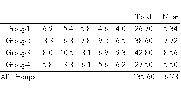
The data in the accompanying table resulted from an experiment run in a completely randomized design in which each of four treatments was replicated five times.

						Total	Mean
Group 1	6.9	5.4	5.8	4.6	4.0	26.70	5.34
Group 2	8.3	6.8	7.8	9.2	6.5	38.60	7.72
Group 3	8.0	10.5	8.1	6.9	9.3	42.80	8.56
Group 4	5.8	3.8	6.1	5.6	6.2	27.50	5.50
All Groups						135.60	6.78

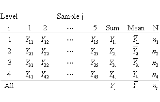
This experiment can be illustrated by the table layout for this 1-way ANOVA experiment shown below: 

The resulting ANOVA table is 

The estimate for the mean of group 1 is 5.34, and the sample size is n₁ = 5. 

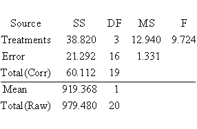
Since the confidence interval is two-sided, the entry a/2 value for the t-table is .5(1 - .95) = .025, and the associated degrees of freedom is N - 4,  or 20 - 4 = 16. 

From t-tables or a computer program we obtain t_.025;16 = 2.120. 

Next we need the standard error of the mean for group 1: 

Hence, we obtain confidence limits 5.34 ± 2.120 (0.5159) and the confidence interval is 

Definition and Estimation of Contrasts

Definitions

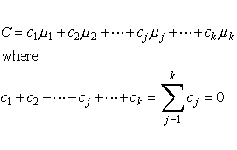
A contrast is a linear combination of 2 or more factor level means with coefficients that sum to zero.

Two contrasts are orthogonal if the sum of the products of corresponding coefficients (i.e. coefficients for the same means) adds to zero.

Formally, the definition of contrast is expressed below, using the notation m_i for the i-th treatment mean: 

Simple contrasts includes the case of the difference between two factor means, such as m₁ - m₂ . If one wishes to compare treatments 1 and 2 with treatment 3, one way of expressing this is by: m₁ + m₂ - 2m_3. Note that 

m₁ - m₂ has coefficients +1, -1 
m₁ + m₂ - 2m₃  has coefficients +1, +1, -2. 
These coefficients sum to zero. 

As an example of orthogonal contrasts note the three contrasts defined by the table below, where the rows denote coefficients for the column treatment means.  The following is true: 

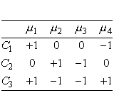
1. The sum of the coefficients for each contrast is zero. 

2. The sum of the products of coefficients of each pair of contrasts  is also 0 (orthogonality property). 

3. The first two contrasts are simply pair wise comparisons, the third one involves all the treatments. 
 

As might be expected, contrasts are estimated by taking the same linear combination of treatment mean estimates. In other words: 

and  Note: These formulas hold for any linear combination of treatment means, not just for contrasts. 
 

Confidence Interval for a Contrast 

An unbiased estimator for a contrast C is given by 

The estimate of  is 

The estimator  is normally distributed because it is a linear combination of independent normal random variables. It can be shown that: 

for the one way ANOVA model under discussion. 

Therefore, the 1-a confidence limits for C are: 

Example 2

We wish to estimate, in our previous example, the following contrast: 

and construct a 95 percent confidence interval for C. 

The point estimate is: 

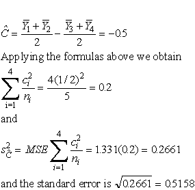
For a confidence coefficient of 95 % and df = 20 - 4 = 16, 
t._025;16 = 2.12. Therefore, the desired 95 % confidence interval is  -.5 ± 2.12(.5158) or 

(-1.594, 0.594).

Estimation of Linear Combinations 

Sometimes we are interested in a linear combination of the factor level means that is not a contrast. Assume that in our sample experiment certain costs are associated with each group. For example there might be costs associated with each factor as follows: 

          Factor      Cost in $ 
               1               3 
               2               5 
               3               2 
               4               1 

The following linear combination might then be of interest: 

This resembles a contrast, but the coefficients c_i do not sum up to zero. A linear combination has definition:  with no restrictions on the coefficients c_i.

Confidence limits for a linear combination C are obtained in precisely the same way as those for a contrast, using the same calculation for the point estimator and estimated variance.