6.
Process or Product Monitoring and Control
6.3.
Univariate and Multivariate Control Charts
6.3.3.
What are Attributes Control Charts?
6.3.3.2.
|
Proportions Control Charts
|
|
|
\(p\) is the fraction defective in a lot or population
|
The proportion or fraction nonconforming (defective) in a
population is defined as the ratio of the number of nonconforming
items in the population to the total number of items in that
population. The item under consideration may have one or more
quality characteristics that are inspected simultaneously. If at
least one of the characteristics does not conform to standard, the
item is classified as nonconforming.
The fraction or proportion can be expressed as a decimal, or, when
multiplied by 100, as a percent. The underlying statistical
principles for a control chart for proportion nonconforming are
based on the binomial distribution.
Let us suppose that the production process operates in a stable
manner, such that the probability that a given unit will not conform
to specifications is \(p\).
Furthermore, we assume that
successive units produced are independent. Under these conditions,
each unit that is produced is a realization of a Bernoulli random
variable with parameter \(p\).
If a random sample of \(n\)
units of product is selected and if \(D\)
is the number of units that are nonconforming, then \(D\)
follows a
binomial distribution
with parameters \(n\) and \(p\)
so that
|
|
The binomial distribution model for number of defectives
in a sample
|
$$ P(D=x) = \left( \begin{array}{c} n \\ x \end{array} \right)
p^x (1-p)^{n-x} \, , \,\,\,\,\,\, x = 0, \, 1, \, \ldots, \, n \, , $$
where
$$ \left( \begin{array}{c} n \\ x \end{array} \right) $$
denotes a "combination", referring to \(n\) things taken \(x\) at a time.
The mean of \(D\) is \(np\)
and the variance is \(np(1-p)\).
The sample proportion nonconforming is the ratio of the
number of nonconforming units in the sample, \(D\),
to the sample size \(n\),
$$ \hat{p} = \frac{D}{n} \, .$$
The mean and variance of this estimator are
$$ \mu = p $$
and
$$ \sigma_{\hat{p}}^2 = \frac{p(1-p)}{n} \, . $$
This background is sufficient to develop the control chart for
proportion or fraction nonconforming. The chart is called the
\(p\)-chart.
|
|
\(p\) control charts for lot proportion defective
|
If the true fraction conforming \(p\)
is known (or a standard
value is given), then the center line and control limits of the
fraction nonconforming control chart is
$$ \begin{eqnarray}
UCL & = & p + 3\sqrt{\frac{p(1-p)}{n}} \\
\mbox{Center Line} & = & p \\
LCL & = & p - 3\sqrt{\frac{p(1-p)}{n}} \, .
\end{eqnarray} $$
When the process fraction (proportion) \(p\)
is not known,
it must be estimated from the available data. This is accomplished
by selecting \(m\)
preliminary samples, each of size \(n\).
If there are \(D_i\)
defectives in sample \(i\),
the fraction nonconforming in sample \(i\)
is
$$ \hat{p}_i = \frac{D_i}{n} \, , \,\,\,\,\, i = 1, \, 2, \, \ldots, \, m \, , $$
and the average of these individuals sample fractions is
$$ \bar{p} = \frac{\sum_{i=1}^m D_i}{mn} = \frac{\sum_{i=1}^m \hat{p}_i}{m} \, . $$
The \(\bar{p}\)
is used instead of \(p\)
in the control chart setup.
|
|
Example of a \(p\)-chart
|
A numerical example will now be given to illustrate the above
mentioned principles. The location of chips on a wafer is measured
on 30 wafers.
On each wafer 50 chips are measured and a defective is defined
whenever a misregistration, in terms of horizontal and/or vertical
distances from the center, is recorded. The results are
|
Sample
|
Fraction
|
Sample
|
Fraction
|
Sample
|
Fraction
|
|
Number
|
Defectives
|
Number
|
Defectives
|
Number
|
Defectives
|
|
|
1
|
0.24
|
11
|
0.10
|
21
|
0.40
|
|
2
|
0.30
|
12
|
0.12
|
22
|
0.36
|
|
3
|
0.16
|
13
|
0.34
|
23
|
0.48
|
|
4
|
0.20
|
14
|
0.24
|
24
|
0.30
|
|
5
|
0.08
|
15
|
0.44
|
25
|
0.18
|
|
6
|
0.14
|
16
|
0.16
|
26
|
0.24
|
|
7
|
0.32
|
17
|
0.20
|
27
|
0.14
|
|
8
|
0.18
|
18
|
0.10
|
28
|
0.26
|
|
9
|
0.28
|
19
|
0.26
|
29
|
0.18
|
|
10
|
0.20
|
20
|
0.22
|
30
|
0.12
|
The reader can download the data as a
text file.
|
|
Sample proportions control chart
|
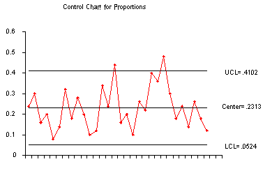
The corresponding control chart is given below:

|


