6. Process or Product Monitoring and Control
6.3. Univariate and Multivariate Control Charts

6.3.1.

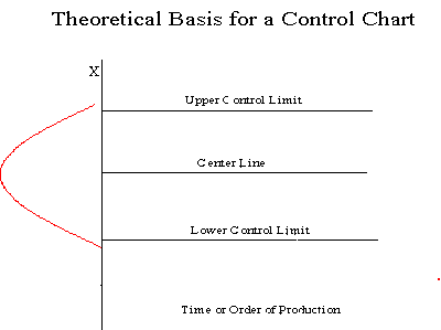
What are Control Charts?

Comparison of univariate and multivariate control data

Control charts are used to routinely monitor quality. Depending on the number of process characteristics to be monitored, there are two basic types of control charts. The first, referred to as a univariate control chart, is a graphical display (chart) of one quality characteristic. The second, referred to as a multivariate control chart, is a graphical display of a statistic that summarizes or represents more than one quality characteristic.

Characteristics of control charts

If a single quality characteristic has been measured or computed from a sample, the control chart shows the value of the quality characteristic versus the sample number or versus time. In general, the chart contains a center line that represents the mean value for the in-control process. Two other horizontal lines, called the upper control limit (UCL) and the lower control limit (LCL), are also shown on the chart. These control limits are chosen so that almost all of the data points will fall within these limits as long as the process remains in-control. The figure below illustrates this.

Chart demonstrating basis of control chart

Why control charts "work"

The control limits as pictured in the graph might be 0.001 probability limits. If so, and if chance causes alone were present, the probability of a point falling above the upper limit would be one out of a thousand, and similarly, a point falling below the lower limit would be one out of a thousand. We would be searching for an assignable cause if a point would fall outside these limits. Where we put these limits will determine the risk of undertaking such a search when in reality there is no assignable cause for variation.

Since two out of a thousand is a very small risk, the 0.001 limits may be said to give practical assurances that, if a point falls outside these limits, the variation was caused be an assignable cause. It must be noted that two out of one thousand is a purely arbitrary number. There is no reason why it could not have been set to one out a hundred or even larger. The decision would depend on the amount of risk the management of the quality control program is willing to take. In general (in the world of quality control) it is customary to use limits that approximate the 0.002 standard.

Letting X denote the value of a process characteristic, if the system of chance causes generates a variation in X that follows the normal distribution, the 0.001 probability limits will be very close to the 3σ limits. From normal tables we glean that the 3σ in one direction is 0.00135, or in both directions 0.0027. For normal distributions, therefore, the 3σ limits are the practical equivalent of 0.001 probability limits.

Plus or minus "3 sigma" limits are typical

In the U.S., whether X is normally distributed or not, it is an acceptable practice to base the control limits upon a multiple of the standard deviation. Usually this multiple is 3 and thus the limits are called 3-sigma limits. This term is used whether the standard deviation is the universe or population parameter, or some estimate thereof, or simply a "standard value" for control chart purposes. It should be inferred from the context what standard deviation is involved. (Note that in the U.K., statisticians generally prefer to adhere to probability limits.)

If the underlying distribution is skewed, say in the positive direction, the 3-sigma limit will fall short of the upper 0.001 limit, while the lower 3-sigma limit will fall below the 0.001 limit. This situation means that the risk of looking for assignable causes of positive variation when none exists will be greater than one out of a thousand. But the risk of searching for an assignable cause of negative variation, when none exists, will be reduced. The net result, however, will be an increase in the risk of a chance variation beyond the control limits. How much this risk will be increased will depend on the degree of skewness.

If variation in quality follows a Poisson distribution, for example, for which np = 0.8, the risk of exceeding the upper limit by chance would be raised by the use of 3-sigma limits from 0.001 to 0.009 and the lower limit reduces from 0.001 to 0. For a Poisson distribution the mean and variance both equal np. Hence the upper 3-sigma limit is 0.8 + 3 sqrt(0.8) = 3.48 and the lower limit is 0 (here sqrt denotes "square root"). For np = 0.8 the probability of getting more than 3 successes is 0.009.

Strategies for dealing with out-of-control findings

If a data point falls outside the control limits, we assume that the process is probably out of control and that an investigation is warranted to find and eliminate the cause or causes.

Does this mean that when all points fall within the limits, the process is in control? Not necessarily. If the plot looks non-random, that is, if the points exhibit some form of systematic behavior, there is still something wrong. For example, if the first 25 of 30 points fall above the center line and the last 5 fall below the center line, we would wish to know why this is so. Statistical methods to detect sequences or nonrandom patterns can be applied to the interpretation of control charts. To be sure, "in control" implies that all points are between the control limits and they form a random pattern.