1.3. EDA Techniques
1.3.5. Quantitative Techniques
1.3.5.1. |
Measures of Location |
- mean - the mean is the sum of the data points divided by
the number of data points. That is,
-
\[ \bar{Y} = \sum_{i=1}^{N}Y_{i}/N \]
The mean is that value that is most commonly referred to as the average. We will use the term average as a synonym for the mean and the term typical value to refer generically to measures of location.
- median - the median is the value of the point which has
half the data smaller than that point and half the data
larger than that point. That is, if X1,
X2, ... ,XN is a random sample
sorted from smallest value to largest value, then the
median is defined as:
-
\[ \tilde{Y} = Y_{(N+1)/2} \;\;\;\;\;\; \mbox{if $N$ is odd} \]
\[ \tilde{Y} = (Y_{N/2} + Y_{(N/2)+1})/2 \;\;\;\;\;\; \mbox{if $N$ is even} \]
- mode - the mode is the value of the random sample that
occurs with the greatest frequency. It is not
necessarily unique. The mode is typically used in
a qualitative fashion. For example, there may be a single
dominant hump in the data perhaps two or more smaller
humps in the data. This is usually evident from a histogram
of the data.
When taking samples from continuous populations, we need to be somewhat careful in how we define the mode. That is, any specific value may not occur more than once if the data are continuous. What may be a more meaningful, if less exact measure, is the midpoint of the class interval of the histogram with the highest peak.
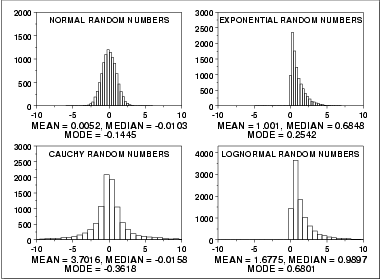
This plot shows histograms for 10,000 random numbers generated from a normal, an exponential, a Cauchy, and a lognormal distribution.

The normal distribution is a symmetric distribution with well-behaved tails and a single peak at the center of the distribution. By symmetric, we mean that the distribution can be folded about an axis so that the 2 sides coincide. That is, it behaves the same to the left and right of some center point. For a normal distribution, the mean, median, and mode are actually equivalent. The histogram above generates similar estimates for the mean, median, and mode. Therefore, if a histogram or normal probability plot indicates that your data are approximated well by a normal distribution, then it is reasonable to use the mean as the location estimator.
The exponential distribution is a skewed, i. e., not symmetric, distribution. For skewed distributions, the mean and median are not the same. The mean will be pulled in the direction of the skewness. That is, if the right tail is heavier than the left tail, the mean will be greater than the median. Likewise, if the left tail is heavier than the right tail, the mean will be less than the median.
For skewed distributions, it is not at all obvious whether the mean, the median, or the mode is the more meaningful measure of the typical value. In this case, all three measures are useful.
For better visual comparison with the other data sets, we restricted the histogram of the Cauchy distribution to values between -10 and 10. The full Cauchy data set in fact has a minimum of approximately -29,000 and a maximum of approximately 89,000.
The Cauchy distribution is a symmetric distribution with heavy tails and a single peak at the center of the distribution. The Cauchy distribution has the interesting property that collecting more data does not provide a more accurate estimate of the mean. That is, the sampling distribution of the mean is equivalent to the sampling distribution of the original data. This means that for the Cauchy distribution the mean is useless as a measure of the typical value. For this histogram, the mean of 3.7 is well above the vast majority of the data. This is caused by a few very extreme values in the tail. However, the median does provide a useful measure for the typical value.
Although the Cauchy distribution is an extreme case, it does illustrate the importance of heavy tails in measuring the mean. Extreme values in the tails distort the mean. However, these extreme values do not distort the median since the median is based on ranks. In general, for data with extreme values in the tails, the median provides a better estimate of location than does the mean.
The lognormal is also a skewed distribution. Therefore the mean and median do not provide similar estimates for the location. As with the exponential distribution, there is no obvious answer to the question of which is the more meaningful measure of location.
Tukey and Mosteller defined two types of robustness where robustness is a lack of susceptibility to the effects of nonnormality.
- Robustness of validity means that the confidence intervals for the population location have a 95% chance of covering the population location regardless of what the underlying distribution is.
- Robustness of efficiency refers to high effectiveness in the face of non-normal tails. That is, confidence intervals for the population location tend to be almost as narrow as the best that could be done if we knew the true shape of the distributuion.
The median is an example of a an estimator that tends to have robustness of validity but not robustness of efficiency.
The alternative measures of location try to balance these two concepts of robustness. That is, the confidence intervals for the case when the data are normal should be almost as narrow as the confidence intervals based on the mean. However, they should maintain their validity even if the underlying data are not normal. In particular, these alternatives address the problem of heavy-tailed distributions.
The mid-range, since it is based on the two most extreme points, is not robust. Its use is typically restricted to situations in which the behavior at the extreme points is relevant.

